3. the external face of maximum size among the set of all embeddings of G with minimum depth. 1 Introduction. A combinatorial embedding Î of a planar graph G ...
Graph Embedding with Minimum Depth and Maximum External Face (Extended Abstract) Carsten Gutwenger1 and Petra Mutzel2 1
Stiftung caesar Ludwig-Erhard-Allee 2, D-53175 Bonn, Germany 2 Vienna University of Technology Favoritenstr. 9–11 E186, A-1040 Vienna, Austria
Abstract. We present new linear time algorithms using the SPQR-tree data structure for computing planar embeddings of planar graphs optimizing certain distance measures. Experience with orthogonal drawings generated by the topology-shape-metrics approach shows that planar embeddings following these distance measures lead to improved quality of the final drawing in terms of bends, edge length, and drawing area. Given a planar graph, the algorithms compute the planar embedding with 1. the minimum depth among the set of all planar embeddings of G, 2. the external face of maximum size among the set of all planar embeddings of G, 3. the external face of maximum size among the set of all embeddings of G with minimum depth.
1
Introduction
A combinatorial embedding Γ of a planar graph G is defined as a clockwise ordering of the incident edges for every vertex with respect to a crossing-free drawing of G in the plane. An equivalent definition of a combinatorial embedding is an ordered list of the boundary edges for each face. A combinatorial embedding Γ together with a given external face f ∈ Γ is called a planar embedding (Γ, f ). A successful approach for generating orthogonal drawings of general graphs is the topology-shape-metrics approach [18,2,6]. Here, in a first step, the crossing structure of the graph is computed. The second step takes this topology as input and produces an orthogonal representation fixing the shape of the drawing. Finally, the third step determines the lengths of the horizontal and vertical edge segments. The goal of the three steps is to minimize the number of crossings, the number of bends, and the total edge length, respectively. Algorithms for the second step typically deal with planar graphs (i.e., the planarized graphs arising in step 1). Such algorithms, in general, need as input a planar embedding (e.g., the bend minimization algorithm by Tamassia [17]). Fortunately, a planar embedding of a planar graph can be computed in linear G. Liotta (Ed.): GD 2003, LNCS 2912, pp. 259–272, 2004. c Springer-Verlag Berlin Heidelberg 2004 �
260
C. Gutwenger and P. Mutzel
time (see [14,5]). However, the choice of the embedding typically has a big impact on the quality of the resulting drawing, and the number of possible embeddings of a planar graph may be exponential in the size of the graph. Since optimizing aesthetic criteria like the number of bends is NP-hard in general [10], finding criteria for planar embeddings that lead to good drawings in practice, as well as efficient algorithms to compute such planar embeddings is desired. Several authors have studied the problem of computing planar embeddings which are optimal with respect to some distance measures. Bienstock and Monma [4] have suggested polynomial time algorithms for computing planar embeddings that minimize the distance measures radius, width, outerplanarity, and face depth. They also showed that it is NP-complete to test whether a planar graph has an embedding with dual diameter bounded above by an input number. Exact algorithms for the NP-hard problem of computing planar embeddings that minimize the number of bends of orthogonal planar graphs have been suggested by Liotta et al. [13] and by Mutzel and Weiskircher [15]. Mutzel and Weiskircher [15] have suggested an exact algorithm for the NP-hard problem of computing a linear cost function on the face cycles. However, all the exact algorithms only work well for graphs with up to 80 edges. In this paper we give linear time algorithms based on the SPQR-tree data structure for computing planar embeddings of planar graphs optimizing various distance measures. Experience in the graph drawing community has shown that planar embeddings following these distance measures lead to improved quality of the final drawing in terms of bends, edge length, and drawing area [1,3,9,16, 20]. The first distance measure is the depth of a planar embedding introduced by Pizzonia and Tamassia [16]. They have suggested an algorithm for a restricted version of computing a minimum depth embedding of a planar graph in which the embeddings of the biconnected components are given and fixed. Our algorithm finds the minimum depth embedding over the class of all planar embeddings without any restriction. The depth of a planar embedding is a measure of the topological nesting of the biconnected components of G in (Γ, f ). For the formal definition, we need to introduce some more terms. A block of G is a biconnected component of G. Given a connected graph, the BC-tree B of G has vertices for each block and each cut vertex of G. There is an edge between a block vertex b associated with a block B and a cut vertex v if v ∈ B. BC-trees are rooted at an arbitrary block of G, and the edges are directed from parent to child (e.g., an edge (v, w)); sometimes they will be considered as undirected (e.g., denoted as {v, w}). Given a planar embedding (Γ, f ) of a planar graph G = (V, E) with face set F , the dual graph G∗ = (V ∗ , E ∗ ) is constructed as follows: V ∗ = F and E ∗ contains an edge {fi , fj } for each e ∈ E such that e is on the boundary of both fi and fj . An extended dual BC-tree of a given planar embedding (Γ, f ) is either the BC-tree of the dual graph G∗ in the case that the edges on the external face do not belong to a single block in G; then, we define r as the (cut) vertex vf ∈ V ∗ associated
Graph Embedding with Minimum Depth and Maximum External Face
3
11
4 10
11
9
9
8 6 7
10 6
7
8
5 1
2
5
4
3
1
2
0
0
(a)
261
(b)
Fig. 1. Two drawings of the same graph given in [16] (computed by the GDToolkit system [11]). The planar embedding in (a) has depth 5, while the one in (b) has depth 1.
with f in G. Otherwise, all edges bordering the external face belong to a unique block B in the dual BC-tree containing the external face vertex vf ∈ V ∗ . Then, the extended dual BC-tree is the dual BC-tree extended by an additional vertex r and the edge (r, b), where b is the block vertex associated with B. Now we are ready to introduce the formal definition of the depth of a planar embedding: For a planar embedding (Γ, f ) of a connected planar graph G, the depth is defined as the height of the extended dual BC-tree with respect to (Γ, f ) rooted at r. The example shown in Figure 1 has already been provided by Pizzonia and Tamassia in order to justify their approach for minimizing the depth. Each of the two drawings has bends and area optimized for its embedding (computed by the GDToolkit system [11]). The planar embedding in Figure 1(a) has depth 5, while the one in Figure 1(b) has depth 1. Obviously, the drawing in Figure 1(b) is much easier to read and to understand than the one in Figure 1(a). Figure 2 shows two drawings of the same graph realizing different planar embeddings. Again, both drawings have the minimal number of bends with respect to their planar embeddings. The drawing in Figure 2(b) looks much more compact than the drawing in Figure 2(a). We observe that the graph is biconnected and hence the depth of any planar embedding is 1. On the other hand, the external face in Figure 2(b) is bordered by 9 edges and is much larger than in Figure 2(a) with only 3 edges. Also the two embeddings in Figure 1 differ in the number of edges contained in the external face. Figure 1(a) has 3 edges bordering the external face, while the better drawing shown in Figure 1(b) has 15. This goes along with our observation that a higher number of edges on the external face leads to improved layout quality. Hence, the second distance measure investigated in this paper is the length of the external face cycle (also called, the size of a face) in the planar embed-
262
C. Gutwenger and P. Mutzel
5 4 3
5 8
7
6
0
2
8
4
1
7
3 6
2
1
0
(a)
(b)
Fig. 2. Two bend-minimal orthogonal drawings of a graph with different planar embeddings.
ding. Our algorithm computes the planar embedding with the external face of maximum size among the set of all possible planar embeddings. The third distance measure considered in this paper is a combination of the first two distance measures: we search the planar embedding with the external face of maximum size among all planar embeddings with minimum depth. We conjecture that this measure provides, in general, the best planar embeddings among the considered distance measures in our paper, and in the literature, leading to improved planar layouts. The rest of the paper is organized as follows. Section 2 provides the required graph-theoretical background. For technical reasons, we describe the algorithm for computing a planar embedding with maximum external face first (see Section 3), before we discuss the two remaining algorithms in Section 4. Because of space restrictions, we have omitted some of the proofs.
2
Preliminaries
SPQR-trees [8,7] basically represent the decomposition of a biconnected graph into its triconnected components. Let G be a biconnected graph. A split pair of G is either a separation pair or a pair of adjacent vertices. A split component of a split pair {u, v} is either an edge (u, v) or a maximal subgraph C of G such that {u, v} is not a split pair of C. Let {s, t} be a split pair of G. A maximal split pair {u, v} of G with respect to {s, t} is such that, for any other split pair {u� , v � }, vertices u, v, s, and t are in the same split component. Let e = (s, t) be an edge of G, called the reference edge. The SPQR-tree T of G with respect to e is a rooted ordered tree whose nodes are of four types: S, P, Q, and R. Each node µ of T has an associated biconnected multi-graph, called the skeleton of µ. Tree T is recursively defined as follows:
Graph Embedding with Minimum Depth and Maximum External Face
263
Trivial Case: If G consists of exactly two parallel edges between s and t, then T consists of a single Q-node whose skeleton is G itself. Parallel Case: If the split pair {s, t} has at least three split components G1 , . . . , Gk , the root of T is a P-node µ, whose skeleton consists of k parallel edges e = e1 , . . . , ek between s and t. Series Case: Otherwise, the split pair {s, t} has exactly two split components, one of them is e, and the other one is denoted with G� . If G� has cut-vertices c1 , . . . , ck−1 (k ≥ 2) that partition G into its blocks G1 , . . . , Gk , in this order from s to t, the root of T is an S-node µ, whose skeleton is the cycle e0 , e1 , . . . , ek , where e0 = e, c0 = s, ck = t, and ei = (ci−1 , ci ) (i = 1, . . . , k). Rigid Case: If none of the above cases applies, let {s1 , t1 }, . . . , {sk , tk } be the maximal split pairs of G with respect to {s, t} (k ≥ 1), and, for i = 1, . . . , k, let Gi be the union of all the split components of {si , ti } but the one containing e. The root of T is an R-node, whose skeleton is obtained from G by replacing each subgraph Gi with the edge ei = (si , ti ). Except for the trivial case, µ has children µ1 , . . . , µk , such that µi is the root of the SPQR-tree of Gi ∪ ei with respect to ei (i = 1, . . . , k). The endpoints of edge ei are called the poles of node µi . Edge ei is said to be the virtual edge of node µi in skeleton of µ and of node µ in skeleton of µi . We call node µ the pertinent node of ei in skeleton of µi , and µi the pertinent node of ei in skeleton of µ. The virtual edge of µ in skeleton of µi is called the reference edge of µi . Let µr be the root of T in the decomposition given above. We add a Q-node representing the reference edge e and make it the parent of µr so that it becomes the new root. Let e be an edge in skeleton(µ) and ν the pertinent node of e. Deleting edge {µ, ν} in T splits T into two connected components. Let Tν be the connected component containing ν. The expansion graph of e (denoted with expansion(e)) is the graph induced by the edges that are represented by the Q-nodes in Tν . We further introduce the notation expansion + (e) for the graph expansion(e) ∪ e. Replacing a skeleton edge e by its expansion graph is called expanding e. The pertinent graph of a tree node µ results from expanding all edges in skeleton(µ) except for the reference edge of µ and is denoted with pertinent(µ). Hence, if e is a skeleton edge and ν its pertinent node, then expansion + (e) equals pertinent(ν). If v is a vertex in G, a node in T whose skeleton contains v is called an allocation node of v. BC-trees and SPQR-trees can be constructed in linear time and use only linear space (see [19,12,8]). They are used to encode all embeddings of a planar connected graph G. Denote with TB the SPQR-tree of a block B ∈ G. The embeddings of B are in one-to-one correspondence with the embeddings of the skeletons of TB . An embedding of B is basically constructed by replacing skeleton edges with their expansion graphs while preserving the embedding. Once all blocks are embedded, an embedding of G is constructed by several applications of the following procedure. Let Γ � be an embedding consisting of a connected union of some blocks. We want to insert a further embedded block ΓB with vertex
264
C. Gutwenger and P. Mutzel
w 0
e
2
f1
f2
4
1
0
4
v Fig. 3. An embedding of expansion + (e) with given vertex lengths. Assuming that e, v, w have length 0, face f1 has size 8 and f2 has size 9, therefore edge e has component length ≥ 9.
c ∈ B ∩ Γ � into Γ � . Then, we have to choose a face containing c as external face of ΓB and insert ΓB into a face of Γ � containing c.
3
Planar Embeddings with Maximum External Face
Let G = (V, E) be a planar connected graph without self-loops. We first consider biconnected graphs and present linear-time algorithms for finding an embedding with maximum external face and for computing the size of a maximum external face containing a prescribed vertex v for every vertex v ∈ V . 3.1
Biconnected Graphs
Let B = (VB , EB ) be a block of G and TB its SPQR-tree. We associate a nonnegative length with each vertex v ∈ B and each skeleton edge � in TB . The length of an edge in B is simply 1. The size of a face f is defined as e∈f length(e) + � v∈f length(v). Consider an edge e = (v, w) in a skeleton graph and let Γe be an embedding of expansion + (e) such that Γe has a face f ∗ containing e of maximum size among all embeddings of expansion + (e). We call such an embedding an embedding of expansion + (e) with maximum length and define the component length of e to be size(f ∗ ) − length(e) − length(v) − length(w) (compare also Figure 3). The general idea of the algorithm is as follows: Let S be a skeleton for which we have chosen an embedding ΓS . In order to extend ΓS to an embedding Γ of B, we have to choose embeddings of the graphs expansion + (e) for all edges e ∈ S. Each face fS in ΓS corresponds to a face fΓ in Γ in which each skeleton edge e ∈ fS is replaced by a path pe on the external face of its expansion graph (see Figure 4). We call this expanding face fS to face fΓ . Vice versa, for each face fΓ� in Γ , we can find a face in a skeleton that can be expanded to fΓ� . Face fΓ is made as large as possible by embedding each expansion graph of an edge in fS , such that the length of the path pe , which we define as the number of edges
Graph Embedding with Minimum Depth and Maximum External Face
265
pe e
fS
fΓ
Fig. 4. A face fS in the skeleton of an R-node (left) and the resulting face fΓ after expanding all edges in fS (right).
in pe plus the lengths of the interior vertices on pe , is the component length of e. We get the following Lemma: Lemma 1. Let B be a planar biconnected graph with vertex lengths and TB its SPQR-tree. Then the following holds: (i) Each skeleton face f can be expanded to a face f � such that the size of f � is the sum of the lengths of the vertices in f plus the component lengths of all edges in f . (ii) There exists an internal node µ ∈ TB and an embedding Γµ of skeleton(µ) such that there is a face f in Γµ that can be expanded to a maximum face f ∗ of B. All edges in f are expanded to expansion graphs with maximum length. We can compute the component length of all non-reference skeleton edges by a bottom-up traversal of TB . Let e be an edge in skeleton(µ) and ν the pertinent node of e. Denote with er the reference edge of ν and with � the sum of the length of the two poles of µ. If we assume that the length of all edges in skeleton(ν) except for er are set to their component length, the component length of e is Q-node: 1 S-node: size of a face in skeleton(ν) minus � P-node: length of the longest edge different from er in skeleton(ν) R-node: size of the largest face containing er in skeleton(ν) minus � Once we have set the length of all non-reference skeleton edges to their component lengths, we can compute the component length of the reference edges by a top-down traversal of TB . Since TB is rooted at a Q-node, the component length of the reference edge of its only son is 1. Consider now a node µ ∈ TB and let S be the skeleton of µ. We assume that the length of each edge in S is set to its component length. We want to compute the component length of the reference edge of each child ν of µ. We distinguish three cases according to the type of µ: S-node: Let L be the sum of the length of all vertices and edges in S. The component length of the reference edge of ν is L minus the length of eS,ν minus the lengths of the two vertices incident to eS,ν .
266
C. Gutwenger and P. Mutzel
P-node: The component length of the reference edge of ν is the length of the longest edge in S different from eS,ν . R-node: Let f be the largest face in S containing eS,ν . The component length of the reference edge of ν is the size of f minus the length of eS,ν minus the lengths of the two vertices incident to eS,ν . According to Lemma 1, we need to find an embedding Γµ of a skeleton with a face f of maximum size among all possible embeddings of skeletons. This can be achieved by inspecting all skeletons S. If S is the skeleton of an R-node, S has only two embeddings which are a mirror of each other. The largest face we can produce is simply a largest face in any embedding of S. If S is the skeleton of a P-node, say a bundle of parallel edges e1 , . . . , ek , we can form any face consisting of two edges ei and ej with i �= j. Hence, the largest face we can produce consists of the two longest edges in S. If S is the skeleton of an S-node, S has only a single embedding consisting of two equally sized faces. This shows that we can find a tree node µ and produce a skeleton face f ∈ Γµ that can be expanded to a maximum face of B. According to Lemma 1, all edges in f have to be expanded to expansion graphs with maximum length, which can be achieved by recursively traversing the tree nodes involved. Theorem 1. Let B = (VB , EB ) be a biconnected planar graph. Then, there exists an O(|VB | + |EB |)-time algorithm that computes a planar embedding of B with maximum external face. In order to compute the size of a maximum external face containing a prescribed vertex v, we have to consider all allocation nodes of v in TB . Suppose we have precomputed the size of all skeleton faces in S- and R-nodes, as well as the length of the two longest edges within a P-node. Then, we can compute the size of a maximum face containing v very efficiently, i.e. in time O(nv + mv ), where nv is the number of allocation nodes of v in TB and mv is the number of skeleton edges in R-nodes incident to representatives of v. Since the size � of TB including all skeleton graphs is linear in the size of B, we know that v∈B (nv + mv ) is linear in the size of B and we get the following lemma. Lemma 2. There exists an O(|VB | + |EB |)-time algorithm that computes the size of a maximum face containing v for every vertex v ∈ VB . 3.2
Connected Graphs
Let B be the BC-tree of G. Consider a block B and a cut-vertex c in G with c ∈ B. If we delete edge {c, B} in B, B is split into two connected components, one component BB containing B. We denote the graph induced by the edges in all blocks contained in BB with Gc,B . The idea of the algorithm is as follows (compare Figure 5): Suppose we have fixed an embedding Γ0 of a block B0 . In order to extend Γ0 to an embedding of G, we have to find an embedding Γc,B with c on its external face for each graph Gc,B with c ∈ B, B �= B0 , and place Γc,B into an adjacent face of c in
Graph Embedding with Minimum Depth and Maximum External Face
f0
B4
267
B1
B5 c1 B3 c2
B2
Fig. 5. A fixed embedding Γ0 of B0 (thick edges), where the graphs Gc1 ,B1 , Gc1 ,B2 and Gc2 ,B5 have been placed into face f0 .
Γ0 . For a fixed face f0 in Γ0 , we can enlarge f0 as much as possible if we place all Γc,B with c ∈ f0 into f0 . We denote with smf B (c) the sum of the sizes of the maximum faces containing c of all Gc,B � with c ∈ B � , B � �= B. If c is not a cut-vertex in G, then smf B (c) is 0. We will use the value smf B (c) as the vertex length of c in B0 and apply the procedures developed in the previous section. The following lemma states the crucial results on which the correctness of our algorithm is based. Lemma 3. (i) Let B be a block of G and define the length of a vertex v in B as smf B (v). If fB is a face in an arbitrary embedding ΓB of B, then there exists an embedding Γ of G with a face f , such that the size of f (disregarding vertex lengths) equals the size of fB . Face f results from embedding each Gc,B � with c ∈ B, B � �= B with a maximum external face containing c and placing it into fB . (ii) Let f be a face in an embedding Γ of G. Then, there exists a block B of G, a length �v for each vertex v ∈ B with �v ≤ smf B (v), and an embedding ΓB of B with a face fB such that the size of f (disregarding vertex lengths) equals the size of fB . Theorem 2. For each block B of G, let smf B (v) be the length of a vertex v ∈ B. Let Bmax be the block having the embedding Γmax with the largest maximum face fmax among all blocks. Then, we can extend Γmax to a planar embedding of G with maximum external face f . Face f results from embedding each Gc,B � with c ∈ Bmax and B � �= Bmax with a maximum external face containing c and placing it into fmax . Proof. According to Lemma 3(i), we will find face f with the required size in an embedding Γ of G. Lemma 3(ii) shows that a maximum face in G cannot be larger than f , hence Γ is an embedding of G with a face f of maximum size. � �
268
C. Gutwenger and P. Mutzel
Algorithm 3.2 shows how to compute a planar embedding with maximum external face. Variable length B (c) stores the length of vertex c in block B, and cstrLength(B, c) is set to the size of a maximum face of Gc,B containing c. Function ConstraintMaxFace(B, c) computes a maximum face in Gc,B containing c and is called for each edge (c, B) ∈ B. Function MaximumFaceRec recursively traverses B from top to bottom. When MaximumFaceRec is called for block B, the length of each vertex v ∈ B is already set to smf B (v). Since the function finally returns the block B ∗ with the largest maximum face of size �∗ , this is the block Bmax in Theorem 2. For embedding each Gc,B with c ∈ B ∗ and B �= B ∗ with a maximum external face containing c, B has to be recursively traversed starting at block B ∗ . Theorem 3. Let G = (V, E) be a planar connected graph. MaximumFace(G) computes a planar embedding of G with maximum external face in time O(|V | + |E|). All algorithms presented in this section can easily be generalized to graphs with predefined non-negative edge lengths, in particular to edges with length 0.
Graph Embedding with Minimum Depth and Maximum External Face B4
B4
B2
269
B3 f3
B2 B1
B3 f3 B7
f1
B7
B6
f1
f4
f2
f4
B5
B1 B5
f0
B6
f2
f0
B0
B0
f0
f0
B0 B4 B2 B5 B7
B0
B2
f1
f3
f4
f2
f1
f3
B1
B3 B6
B1
B5 B7
B3
B4
f4 B6
Fig. 6. Two different extensions of an embedding Γ0 of a block B0 with their corresponding block-cutface trees.The left extension has depth 3 whereas the right one has depth 5.
4
Planar Embeddings with Minimum Depth
Let G = (V, E) be a planar graph. Consider a block B with planar embedding ΓB . An extension of ΓB denotes a planar embedding of G which results from embedding all graphs Gc,B � with c ∈ B and B � �= B so that c lies on the external face and placing them into a face of ΓB . Let mc,B � be the minimum depth of a planar embedding of Gc,B � with c on the external face. We define further mB (c) := max{0} ∪ {mc,B � | c ∈ B � , B � �= B} mB := max mB (c) c∈B
MB := {c ∈ B | mB (c) = mB } Then, the minimum depth of an extension of an embedding of B is mB if there is an embedding of B in which all vertices in MB lie in a common face, and mB + 2 otherwise (compare Figure 6). The following lemma shows the relationship between minimizing the depth and maximizing the external face. Lemma 4. Set the length of all edges in B to 0 and the length of a vertex v in B to 1 if v ∈ MB , and 0 otherwise. Let (Γ ∗ , f ∗ ) be a planar embedding of B with maximum external face f ∗ . Then, the minimum depth of an extension of an embedding of B is
270
C. Gutwenger and P. Mutzel
mB
if size(f ∗ ) = |MB |
mB + 2 otherwise The problem of finding a planar embedding of a graph Gc,B with minimum depth such that c is on the external face can be tackled the same way. Based on this result, algorithm MinimumDepth proceeds similar to algorithm MaximumFace for connected graphs. First, the values mc,B for all edges (c, B) in the BC-tree B are computed by a bottom-up traversal of B. The length of each vertex v �= c in B is set according to Lemma 4 and a maximum face in B is computed that contains c. Afterwards, B is traversed from top to bottom. When a block B = (VB , EB ) is visited, the values mc,B � are already computed for each cut-vertex c in G that is contained in B. According to Lemma 4, we set the vertex lengths in B and compute the minimum depth of an extension of B by finding a maximum face in B. Before we proceed with the descendants of B in tree B, we have to compute the values mc,B for all edges (B, c) ∈ B. We distinguish two cases: MB = {c1 , . . . , ck } with k ≥ 2: We compute a maximum face in block B containing c using the vertex lengths we have already assigned. MB = {c}: In this case, m2 = maxv∈VB ,v�=c mB (v) is less than mB and we cannot reuse the vertex lengths. However, this case can occur at most once for a block which allows us to invest O(|B|) running time. We calculate new vertex lengths according to M2 = {c ∈ VB \ {v} | mB (c) = m2 } and find a maximum face in B containing c using these vertex lengths. Since MaximumFace and MinimumDepth proceed in a similar fashion, it is possible to combine both algorithms to a new algorithm MinDepthMaxFace that computes a planar embedding with maximum external face among all planar embeddings with minimum depths. This can be achieved by using a pair (d, �) as length attribute, where the first component d refers to the 0 − 1 length attribute used in MinimumDepth and � refers to the length attribute used in MaximumFace. The linear order on these tuples is defined componentwise, i.e. (d, �) > (d� , �� ) ⇐⇒ d > d� or (d = d� and � > �� ) Each time a maximum face in a block has to be computed, we first determine a maximum face according to the linear order defined above. If the resulting maximum face has size (d∗ , �∗ ) and d∗ is the number of cut-vertices we want to place in a common face (e.g. d∗ = |MB | as in Lemma 4), we also have found a planar embedding with a maximum face among all planar embeddings with minimum depth. Otherwise, the value d∗ is irrelevant since all extensions will have the same depth and there might be planar embeddings with a larger external face. Therefore, we call the procedure for finding a maximum face in a block again, this time respecting only the second component � of the length attribute.
Theorem 4. Let G = (V, E) be a planar connected graph.
Graph Embedding with Minimum Depth and Maximum External Face
271
i) Algorithm MinimumDepth(G) computes a planar embedding of G with minimum depth. ii) Algorithm MinDepthMaxFace(G) computes a planar embedding of G with maximum external face among all planar embeddings of G with minimum depth.
References [1] C. Batini, E. Nardelli, and R. Tamassia. A layout algorithm for data-flow diagrams. IEEE Trans. Soft. Eng., SE-12(4):538–546, 1986. [2] C. Batini, M. Talamo, and R. Tamassia. Computer aided layout of entity relationship diagrams. The Journal of Systems and Software, 4:163–173, 1984. [3] C. Batini, M. Talamo, and R. Tamassia. Computer aided layout of entityrelationship diagrams. Journal of Systems and Software, 4:163–173, 1984. [4] D. Bienstock and C. L. Monma. On the computational complexity of embedding planar graphs to minimize certain distance measures. Algorithmica, 5(1):93–109, 1990. [5] N. Chiba, T. Nishizeki, S. Abe, and T. Ozawa. A linear algorithm for embedding planar graphs using PQ-trees. J. Computer and System Sciences, 30:54–76, 1985. [6] G. Di Battista, P. Eades, R. Tamassia, and I. G. Tollis. Graph Drawing. Prentice Hall, 1998. [7] G. Di Battista and R. Tamassia. On-line maintanance of triconnected components with SPQR-trees. Algorithmica, 15:302–318, 1996. [8] G. Di Battista and R. Tamassia. On-line planarity testing. SIAM J. Comput., 25(5):956–997, 1996. [9] Didimo and Liotta. Computing orthogonal drawings in a variable embedding setting. In K. Chwa, editor, Algorithms and Computation (Proc. ISAAC ’98), volume 1533 of LNCS, pages 79–88. Springer-Verlag, 1998. [10] A. Garg and R. Tamassia. On the computational complexity of upward and rectilinear planarity testing. SIAM J. Computing, 31(2):601–625, 2002. [11] Graph drawing toolkit: An object-oriented library for handling and drawing graphs. http://www.dia.uniroma3.it/ gdt. [12] C. Gutwenger and P. Mutzel. A linear time implementation of SPQR trees. In J. Marks, editor, Graph Drawing (Proc. GD 2000), volume 1984 of LNCS, pages 77–90. Springer-Verlag, 2001. [13] G. Liotta, F. Vargiu, and G. Di Battista. Orthogonal drawings with the minimum number of bends. In Proceedings of the 6th Canadian Conference on Computational Geometry, pages 281–286. University of Saskatchewan, 1994. [14] K. Mehlhorn and P. Mutzel. On the embedding phase of the Hopcoft and Tarjan planarity testing algorithm. Algorithmica, 16(2):233–242, 1996. [15] P. Mutzel and R. Weiskircher. Bend minimization in orthogonal drawings using integer programming. In O. H. Ibarra and L. Zhang, editors, Proceedings of the Eighth Annual International Conference on Computing and Combinatorics (COCOON 2002), volume 2387 of LNCS, pages 484–493. Springer-Verlag, 2002. [16] M. Pizzonia and R. Tamassia. Minimum depth graph embedding. In M. Paterson, editor, Algorithms – ESA 2000, volume 1879 of LNCS, pages 356–367. SpringerVerlag, 2000.
272
C. Gutwenger and P. Mutzel
[17] R. Tamassia. On embedding a graph in the grid with the minimum number of bends. SIAM J. Comput., 16(3):421–444, 1987. [18] R. Tamassia, G. Di Battista, and C. Batini. Automatic graph drawing and readability of diagrams. IEEE Trans. Syst. Man Cybern., SMC-18(1):61–79, 1988. [19] R. E. Tarjan. Depth-first search and linear graph algorithms. SIAM J. Comput., 1(2):146–160, 1972. [20] R. Weiskircher. New Applications of SPQR-Trees in Graph Drawing. PhD thesis, Universit¨ at des Saarlandes, 2002.