Keywords: CUDA; GPGPU; graph generation; dynamic memory allocation. 1. ...... [4] D. B. Johnson, âFinding all the elementary circuits of a directed graph,â.
Graph Generation on GPUs using Dynamic Memory Allocation A. Leist and K.A. Hawick Science, Massey University 2 Albany, North Shore 102-904, Auckland, New Zealand 1 Computer
Abstract— Complex networks are often studied using statistical measurements over many independently generated samples. Irregular data structures such as graphs that involve dynamical memory management and “pointer chasing” are an important class of application and have attracted recent interest in the form of the Graph500 benchmark formulation. The generation of simulated sample network graphs and measurement of their properties can be accelerated using Graphical Processing Units (GPUs) and we discuss some algorithmic approaches using Compute Unified Device Architecture (CUDA). We particularly discuss recent support for dynamic memory allocation within CUDA GPU code and present some performance data for Watts’ α small-world network model. Keywords: CUDA; GPGPU; graph generation; dynamic memory allocation
1. Introduction Generating synthetic graph or network data is very useful in investigating the statistical properties of various models. Properties such as the average path length [1], [2], clustering coefficient [3]; circuit and loop structure [4]; between-ness and reachability of the networks defined by various models can all be measured quantifiably on various sample network realisations. Scaling can be studied as the size of the generated synthetic data set is varied and for some models other parameters can also be varied and their effect systematically studied. This is a powerful approach as real data from experiments, real physical systems or surveys often contain noise or inaccuracies whereas a comparison with synthetic data – particularly when averaged over many samples – can make it a lot easier to identify effects and make comparisons with theoretical predictions. A great deal of work has been reported in the literature on the properties of complex networks [5], [6]. These include: classic random graphs [7], [8]; small-World graphs such as the Watts-Strogatz β-model [9] and scale-free and preferential attachment models such as that of Barab´asi and Albert [10]. Applications include social problems like collaboration networks [11]; clustering and community structure determination [12]; and the Internet [13] and world-wide web [14]. An interesting model that has attracted somewhat less effort is Watts’ α-model. This sociological model presents some challenging computational problems in generating large synthetic sample networks. A sample network generated with the α-model is illustrated in Figure 1. Investigation of the properties of small-world networks [15], [16] reveals that many of the interesting phenomena are only revealed over size scales that vary with some power law. Consequently it is necessary to generate networks with a large number of nodes with potentially large numbers of edges as well. This is computationally challenging and parallel computing techniques become necessary just to generate good sample sizes of large synthetic networks.
Parallel graph generation has attracted recent interest due to the announcement of the Graph500 benchmark [17] for supercomputer systems in 2010. Led by Murphy at the Sandia National Laboratory, the Graph500 is an important attempt to recognise that many of the application problems that are run on supercomputers are not necessarily well characterised by the linear algebra problem represented by the widely quoted Linpack benchmark, which is used to compile the Top500 [18] list of worldwide supercomputers. The Graph500 benchmark is still in an early stage of uptake and adoption and consists of a two-part benchmark to generate a scale-free graph and to perform parallel searches upon it. The synthetic graphs can be quite large in size and the scalability of performance with graph size is an important aspect of this sort of performance benchmark. We have chosen to study algorithms for generation of Watts α-model networks on data-parallel accelerator devices such as graphical processing units (GPUs). There has been a great deal of interest in the performance and capabilities of GPUs in recent years and several of the top performing supercomputers in the Top500 list in fact employ GPU accelerators to attain their performance ratings with Linpack. It therefore is of topical interest to explore the performance of GPUs in carrying out graph generation and in particular to determine how well some recent features of GPU programming models and systems cope with these tasks. We explore the performance of GPUs using NVIDIA’s Compute Unified Device Architecture (CUDA) and in this paper we look at a recently introduced CUDA capability – to allocate memory dynamically within the GPU code itself. The programming model for GPUs has until recently been that of calling compute kernels written in CUDA to run on the GPU as ”pseudo subroutines” from the conventional CPU host program. Memory management had to be performed in the CPU calling code only. The recent introduction [19] of the malloc and free routines into CUDA offers some new possibilities for dynamical memory ”pointer-chasing” applications such as graph generation. Our article is structured as follows. In Section 2 we define the Watts α-model and summarise the generation algorithm for synthetic networks of this type. The relevant features of the CUDA GPU architecture are described in Section 3. In Section 4 we expand on details of our serial and parallel implementations of the model using single and multi-core CPU approaches as well as a GPU implementation. We present some scaling and performance results in Section 5 and a discussion of their implications in Section 6. We offer some conclusions and areas for further work with multi-core and GPU graph generation algorithms in Section 7.
2. The α-Model Watts introduced the α-model as a way of interpolating between the two extreme social network cases of the “caveman” model and “solaris” model [9]. The “cave-man” model
α = a tunable parameter, 0 0 i,j k p, mi,j = 0
(1)
where: Ri,j = a measure of vertex i’s propensity to connect to vertex j (zero if they are already connected) mi,j = number of vertices adjacent to both i and j k = the average degree of the graph p = a baseline, random �−1 probability of an edge (i, j) existing (p � n2 )
GPU architectural details have been described in detail elsewhere [21] but for completeness we give here a brief summary of memory and other architectural features critical to an explanation of our graph generation algorithm. Of the many GPGPU APIs available [19], [22], [23], [24], NVIDIA’s CUDA stands out as the most developed and advanced API. However, it can only be used in conjunction with NVIDIA GPUs. Our development of GPGPU applications uses the CUDA toolkit and is thus limited to graphics hardware from the same manufacturer. While we specifically discuss the NVIDIA device architecture, most of the concepts are transferable to products from other vendors. CUDA compliant GPUs contain a scalable array of Streaming Multiprocessors (SMs), which in turn are host to up to 32 Scalar Processors (SPs) in the latest generation of “Fermi”-architecture based devices. Each SM can perform computation independently but the SP cores within the same multiprocessor all execute instructions synchronously. NVIDIA call this paradigm Single Instruction Multiple Thread (SIMT) [19]. The GPU hardware is capable of managing thousands of threads at a time. It performs the tasks of creating and scheduling threads in hardware, which keeps the overhead of managing a large number of threads very small. The GPU is designed to support fine-grained parallelism. In order to utilise the hardware properly, applications need to split the work load into many threads, each of which performs a relatively small unit of work. GPUs contain several different types of memory. The latest generation of Fermi devices even adds an implicit L1/L2 cache hierarchy to the mix, a feature previously not available on GPUs. The GPU memory types explicitly accessible from CUDA are as follows [19]: Registers are used to store local variables belonging to each thread. When registers can not hold all local variables, then they spill into Local Memory, which is an area of the L1/L2 caches on Fermi devices and a section of much slower device memory on older GPUs. Global Memory is the largest section of memory and also resides in device memory. It is the only memory type that the CPU can read from and write to. It is accessible by all threads, but has the slowest access times (400-600 clock cycles). The total transaction time can be improved by coalescing – 16 sequential threads that access 16 sequential and word-aligned memory addresses can coalesce the read/write into a single memory transaction. Shared Memory is a fast on-chip read/write memory that can be used as an explicit cache and to share data between threads in the same thread block. Provided that threads access different memory banks (16 for pre-Fermi devices and 32 for Fermi devices), memory transactions are as fast as accessing registers. Texture Memory is a cached method for reading from a section of global
memory that is bound to a texture reference. Texture memory is optimised for spatial memory access. It performs best when streaming data that is located spatially close in the dimensions defined by the texture reference. Constant Memory is another cached method for reading from global memory. A global memory read is only required in the event of a cache miss. If all threads read the same value from the constant cache, the cost is the same as reading from registers. The developer must explicitly utilise the memory types best suited for the given task. Because bandwidth is limited, the optimal memory access strategy can provide huge performance gains, and the wrong strategy can severely hamper performance. A CUDA application has a number of threads organised into thread blocks, which are all arranged into a grid. A block of threads has up to three dimensions (x,y,z) and can contain no more than 512 (1024 on Fermi devices) threads. A grid has two dimensions (x,y) and has a maximum size of 65535 in each dimension. CUDA allows the user to control the arrangement of threads into blocks and of blocks into the grid. The developer can control how these threads are arranged in order to make optimal use of the on-chip memory. When a CUDA application is executed, each block is assigned to execute on one multiprocessor. This SM will manage and execute the threads within the block on its SPs. While the block arrangement does not have a significant impact on the execution of the threads on the multiprocessors, it strongly affects the manner in which threads access memory and use the memory optimisations available on the GPU. Threads should be arranged into blocks such that the maximum amount of data can be shared between threads in fast on-chip memory and that any unavoidable global memory accesses be coalesced.
4. Generating Complex Networks Complex networks arising from generator algorithms like the α model have non-trivial topological features, like those often found in real-world networks such as social networks [25], [11], metabolic networks [26], [27] or neural networks [28]. The connections between nodes in a complex network are neither purely regular nor purely random. Many of these networks possess the properties of high clustering and short mean vertex-vertex path length characteristic to small-world networks [9], which explains the interest in this category of networks over the last decade. As can be seen from the algorithm in Section 2 above, there are some compute-intensive stages involved in generating αmodel synthetic networks. The O(n2 k) complexity of the algorithm arises from the need to compute a property over all vertices for each edge of each vertex. It is therefore attractive to find a way of accelerating or parallelising the algorithm to allow feasible simulation of networks with large n and k. We have implemented the α-model for and compare the performance between: a single CPU core (Section 4.1), a multi-core CPU utilising all available cores (Section 4.2) and a graphics device used as compute accelerator (Section 4.3).
4.1 The Sequential CPU Implementation The sequential CPU implementation is used as reference to measure the scaling behaviour of the multi-threaded implementation and to explain the basic steps of the algorithm. Algorithm 1 uses pseudo-code to describe the steps that are executed when generating a graph using the α-model.
Algorithm 1 Pseudo-code for the sequential CPU implementation of Watts’ α-model network generator. //generate M ← kn/2 edges for e ← 1 to M do //R is the set of vertices not yet chosen in this round if R = {} then R ← init. remaining vertices to set of all vertices V vi ← randomly chosen vertex from R remove vi from R for all vj ∈ V, j 6= i do p ← pbase × uniform random number determine if edge ei,j exists count the neighbours shared by vi and vj P [j] ← compute vi ’s propensity to connect to vj normalise the results in P //select vi ’s new neighbour vj r ← uniform random number psum ← 0.0 for all vj ∈ V, j 6= i ; psum < r do psum ← psum + P [j] insert vj into adjacency-list Ai of vi insert vi into adjacency-list Aj of vj
The propensity Ri,j of vertex vi to connect to vertex vj ∈ V, j 6= i is calculated according to Equation 1. The baseline, �−1 random probability of an edge existing is pbase = n2 . To account for the p � pbase in the equation, the probability p is calculated for every possible edge ei,j by multiplying the baseline probability with a uniform random number. All implementations of the generator described here insert a new neighbour into an adjacency-list so that the list is sorted in ascending order. This significantly improves performance when counting the neighbours shared by two vertices.
4.2 The Multi-Threaded CPU Implementation While CPU manufacturers have traditionally increased the CPU frequencies from one generation to the next, this trend has slowed down dramatically over the last years, as the increasing power consumption becomes more and more difficult to manage. Manufacturers like Intel or AMD have instead started to incorporate more cores onto a single CPU die. The consequence for software developers and end users is that sequential software does not automatically run faster on newer CPUs. Programmers have to re-think and modify their software to utilise multiple threads that can run concurrently on different CPU cores. However, multi-threaded programming is more difficult than writing a sequential implementation. To ease the burden placed on the developers and to increase their productivity, libraries have emerged that attempt to abstract some of the difficulties of multithreaded programming away from the developer. One of these libraries is the Threading Building Blocks (TBB) library [29] developed by Intel. We have shown previously [30] that it achieves comparable performance to low-level multi-threaded implementations based on POSIX threads [31]. We have used TBB to parallelise the CPU implementation of the α-model. To achieve good performance, the inner-loops need to be parallelised where possible. The following loops described in Algorithm 1 can be executed in parallel: • The set R of vertices not yet chosen in the current round is initialised using tbb::parallel for. • The random numbers needed for p ← pbase × uniform random number are generated using T instances of tbb:tbb thread, where T is the number of logical CPU cores available. Each thread generates n/T random numbers using its own random number generator (RNG) instance to ensure repeatability of the algorithm. The
Algorithm 2 Propensity computation using TBB’s tbb::parallel reduce. This code uses the lambda expressions introduced in the upcoming C++0x standard. Lambda expressions let the compiler do the work of creating the function objects needed by TBB, which makes the code easier to read. Each task iterates over a range of values, computing the respective propensity values. double t o t a l P r o p e n s i t y = tbb : : p a r a l l e l r e d u c e ( t b b : : b l o c k e d r a n g e (0 , n V e r t i c e s ) , 0 . 0 , [ = ] ( c o n s t t b b : : b l o c k e d r a n g e & r a n g e , d o u b l e i n i t )−>d o u b l e { / / t h i s lambda f u n c t i o n c o m p u t e s t h e / / p r o p e n s i t i e s f o r a range of v e r t i c e s d o u b l e sum = i n i t ; / / sum o v e r g i v e n r a n g e c o n s t i n t end = r a n g e . end ( ) ; f o r ( i n t i = r a n g e . b e g i n ( ) ; i < end ;++ i ) { / / compute p r o p e n s i t y [ i ] here sum += p r o p e n s i t y [ i ] ; / / add t o sum } r e t u r n sum ; }, [ ] ( d o u b l e x , d o u b l e y)−>d o u b l e { / / lambda f u n c t i o n c o m b i n e s two r e s u l t s r e t u r n x+y ; } );
random numbers are stored in an array for consumption in the next step. Repeatability is also the reason why the random numbers are not generated as part of the following tbb:parallel reduce step. The TBB scheduler assigns the tasks used during the reduction operation dynamically to hardware threads and does not expose this information to the developer, making it difficult to generate the same sequence of random numbers over multiple runs initialised with the same seed. • The most time consuming loop by far is the computation of vi ’s propensity to connect to all vj ∈ V . It is however fairly straight forward to parallelise, as there are no dependencies between the iterations except for the calculation of the total propensity sum, which is later on needed to calculate the uniform propensity values. This can be implemented using the tbb::parallel reduce operation as shown in Algorithm 2. The last remaining inner-loop iterates over the propensity values, normalises these values and computes the inclusive prefix-sum until a random number exceeds the sum, at which point it has found the new neighbour vj and can stop running. This loop is computationally cheap, runs for only n/2 iterations on average, would require a parallel scan over all n elements and another parallel operation to determine vj and is therefore not worth parallelising on the CPU. The two function calls needed to create the new edge by inserting the two vertices into each others adjacency-lists (vj into Ai and vi into Aj ) can be executed in parallel using tbb::parallel invoke. However, this decreased performance slightly during our tests and is thus not done in parallel.
4.3 The CUDA GPU Implementation Graphical processing units have become popular as compute accelerators for non-graphical applications in the highperformance computing sector over the last years. NVIDIA has helped this trend with their popular CUDA toolkit, which
Algorithm 3 Pseudo-code for the CUDA implementation of Watts’ α-model network generator. This is the host code that manages the CUDA execution. allocate device memory incl. sufficient heap memory generate seeds for the device RNGs and copy to device do in parallel on the device using T threads: initialise device RNGs Vdeg ← 0 //init. the vertex degree device array create CUDPP plan for parallel scan on the device //generate M ← kn/2 edges for e ← 1 to M do //R is the set of vertices not yet chosen in this round if R = {} then R ← init. remaining vertices to set of all vertices V vi ← randomly chosen vertex from R remove vi from R do in parallel on the device using T threads: generate n random numbers do in parallel on the device using n threads: call compute propensity kernel do in parallel on the device using n threads: call normalise propensity kernel do in parallel on the device: call cudppScan (inclusive prefix-sum) do in parallel on the device using n threads: call select nbr kernel do in parallel on the device using 2 thread blocks: call add arc kernel destroy CUDPP plan and free device memory
introduces a few extensions to C++ that enable developers to tap into the processing power of the GPU using well established C programming tools and skills. The GPU code is written in form of so called device kernels – routines that execute on the GPU – which are managed by the CPU running the host program. The CPU is free to perform other tasks while the GPU is processing a kernel. The GPU has a highly data-parallel architecture with many processing units, making it very powerful when executing the same instructions on large arrays of data, but making it difficult to achieve good performance when running algorithms that are more serial in nature, have many conditional branches or are bandwidth-limited. However, we have shown [32], [30], [33], [21] that it is often possible to achieve good speed-ups over traditional CPUs even in such less-thanoptimal situations. The task of generating a graph like the α-model is particularly challenging, as it is necessary to repeatedly iterate over the neighbours structure, which puts high demands on the memory bandwidth and does not perform many compute instructions per data element. But the recent interest in the Graph500 and the newly gained ability to dynamically allocate and free memory in device code makes it an interesting challenge. Algorithm 3 describes the host code that coordinates the device kernel execution. We use Marsaglia’s random number generator [34] to generate both the host and device random numbers. The CUDA implementation of the RNG is explained in [35]. For large networks it would not be feasible to have a separate RNG instance for every vertex, as each instance requires 400 bytes of global memory. We therefore use a specialised RNG kernel, which is executed by T CUDA threads, to generate the random numbers. Every thread generates x random numbers per kernel call, where x = ceil(n/T ). The value of T depends on the graphics hardware used. It must be large enough to keep the device busy and it should be divisible by the number of cores available on the GPU, the number of multiprocessors and the thread block size. We set T = 30720 for the GTX580 used for the performance measurements reported in this paper.
Algorithm 4 The compute propensity kernel. Input parameters: vi , pbase , alpha, k vj ← global thread ID queried from CUDA runtime sums ← 0.0 //init. block local propensity sum p ← pbase × (random uniform number) ki ← load degree of vertex vi Ai (ptr) ← load the pointer to adjacency-list Ai Ai ← load adjacency-list at Ai (ptr) into shared memory synchronise thread block determine if edge ei,j exists (vj ∈ Ai ) if edge does not exist then kj ← load degree of vertex vj Aj (ptr) ← load the pointer to adjacency-list Aj count the neighbours shared by vi and vj p ← compute vi ’s propensity to connect to vj sums [btid] ← p //btid is the thread idx within the block P [vj ] ← p //write propensity to global memory synchronise thread block sums ← perform reduction operation //sums [0] now contains the block local sum if btid = 0 then atomically add the local sum sums [0] to the global sum
Algorithm 5 Device function countSharedNbrs counts the number of neighbours shared by two vertices. It assumes that the adjacency-lists are sorted in ascending order. The performance of this function is critical to the overall performance. Ai is stored in shared memory. device forceinline Uint countSharedNbrs ( int v i , int ∗ A i , int v j , int∗ A j ) { Uint count = 0; f o r ( i n t i d x 1 =0 , i d x 2 =0 , tmp ; i d x 1 0 then free memory pointed to by Av old (ptr)
cudppScan, a function of the CUDA Data Parallel Primitives Library [36] (CUDPP), which performs an inclusive parallel prefix-sum operation on the input data. The result of the scan operation is the array Pi,j , ∀j 6= i of subintervals in the range [0, 1). This is passed to select nbr kernel, along with a uniform random number. The kernel, described in Algorithm 6, then determines for every vj if the random number falls into the respective subinterval. To do this, each thread checks whether the random number is larger than or equal to the upper end of the propensity range for the previous vertex P [vj − 1] and smaller than the upper end of the propensity range P [vj ]. This is the case for exactly one vertex vj , which is selected as the new neighbour. Finally, the edge ei,j can be created. This is done in Algorithm 7 add arc kernel. This kernel is only executed by 2 thread blocks, one for each end of the new edge, which it inserts into the respective adjacency-list. This only utilises a fraction of the processing units on the device (16 multiprocessors with a total of 512 processing units on the GTX580). To improve device utilisation, we use two CUDA streams to concurrently run the add arc kernel and generate the random numbers needed for the next iteration. These two kernels have no dependencies on each other and can therefore safely run in parallel. The add arc kernel does not allocate new memory every time it adds a new vertex. Instead, it increases the allocated length by 32 elements when needed. This is critical to performance, as the malloc operations are expensive. The minimum increment should be 4 for 32-bit arrays, as the pointers returned by malloc are aligned to 16 bytes. However, 32 works nicely with the 128 byte cache line width on Fermi devices and performed better in our experiments. The downside of allocating too much is wasted memory. We will refer to this CUDA implementation as CUDA 1. We have also implemented a second version of the algorithm, which we shall refer to as CUDA 2 respectively, that is identical to the first implementation except for one key criterion: It replaces the add arc kernel with a kernel that merely determines the indices into the adjacency-lists at which the new neighbours have to be inserted to keep them sorted. The indices are written to mapped host memory. The actual memory allocation, deallocation and copying is initiated in the traditional way by the host thread with calls to cudaMalloc, cudaFree and cudaMemcpy(Async).
Fig. 2: This plot shows how the algorithms scale with the network size n = 20 000 to 100 000. The mean degree is set to k = 20 and α = 1.0. The standard deviations showing the measurement error are smaller than the symbol size.
Fig. 3: This plot shows how the algorithms scale average degree k = 20 to 100. The network size n = 20 000 and α = 1.0. The standard deviations the measurement error are smaller than the symbol
This second implementation is used to compare the performance of the new in-kernel functions for dynamic memory management to the library calls initiated by the host thread.
fixed increment size of 32 elements for the adjacency-list lengths. The host library calls for memory management have a much smaller impact on the overall performance, and for that reason the results for CUDA 2 do not show the same anomalies. CUDA 2 is 1.51 times faster than the TBB implementation and 10.83 times faster than the sequential CPU implementation. These speed-ups are not as impressive as those seen for more regular or compute heavy algorithms, but the results show that the GPU can still consistently outperform the CPU even for a graph generator problem like the one described here. The new device code malloc() and free() functions, while arguably more elegant, have been shown to be significantly more expensive than the proven method of handing device memory management tasks to the host.
5. Performance Results To compare the performance of the different implementations of the α-model, we measured the execution time for each of the algorithms. We tested the scaling behaviour with increasing network size and fixed degree and vice versa. The parameter α is always set to 1.0 for these experiments. Other values of α only have a very minor impact on the performance. The test platforms run Ubuntu Linux 10.10 with GCC 4.5 and CUDA 3.2. Both the single-threaded and multi-threaded CPU implementations were tested on an Intel Core i7 970 with 6 cores running at 3.2 GHz. This machine has 12 Gbytes of main memory. The CUDA algorithm was tested on an Intel Core i7 870 with 4 cores running at 2.93 GHz, 4 Gbytes of main memory and an NVIDIA GTX 580 GPU. Figure 2 compares the performance with increasing network size and fixed degree k = 20. For the largest measured network size n = 100 000, the multi-core TBB implementation runs 5.42 times faster than the sequential algorithm and thus scales well with the number of cores. The GPU implementation CUDA 1 runs 1.75 times faster than the TBB implementation and 9.50 times faster than the sequential CPU code. Implementation CUDA 2 is 2.33 times and 12.64 times faster than the sequential and TBB CPU implementations respectively. Figure 3 compares the performance with increasing degree and fixed network size n = 20 000. For the largest degree k = 100, the multi-core TBB implementation runs 7.16 times faster than the sequential implementation. Intel’s HyperThreading Technology allows each physical processor core to appear as two logical cores and to work on two tasks at the same time, improving the utilisation of the physical core and increasing throughput. The speed-up value shows that this technology can pay-off, allowing the algorithm to achieve performance values higher than possible by the increase of physical cores alone. At this degree, the TBB implementation even slightly outperforms implementation CUDA 1 running on the graphics device by 1.03 times. The small kinks in the performance scaling of CUDA 1 are caused by the
with the is set to showing size.
6. Discussion The addition of new features like dynamic memory allocation in device code makes CUDA an increasingly powerful environment that enables programmers to tap into the parallel processing power of today’s graphics processing units. And while GPUs have received lots of attention for their impressive number crunching capabilities, which have enabled GPU based supercomputers to take up the top spots in the TOP500 benchmark, they are not always seen as the best choice when it comes to memory bound or irregular problems. However, such algorithms are essential for a wide variety of applications, and the introduction of the Graph500 highlights the importance of graph based algorithms for high performance computing. While it is true that the speed-ups achieved for many graph based algorithms are not as impressive as those for compute bound algorithms, we have shown time and time again that they can still be very respectable if the code and data structures are optimised for the GPU hardware. The graph generation problem discussed in this article again proves this point. As shown in Table 1, the GPU manages to consistently outperform a high-end six core Intel CPU of the same vintage when managing the device memory from the host (CUDA 2) and at least keeps up with the multithreaded CPU implementation when using in-kernel dynamic memory management (CUDA 1). A high connectivity in the α-model algorithm is particularly taxing for the graphics
Table 1: Summary of the performance results. The speedup values are relative to the respective sequential CPU implementation and the quoted slopes are for the least squares linear fits to the data sets. Compute Device Speed-up n=100,000 ; k=20 ; α=1.0 Core i7 970 (1 core) 1.00 Core i7 970 (6 cores) 5.42 GTX 580 - CUDA 1 9.50 GTX 580 - CUDA 2 12.64 n=20,000 ; k=100 ; α=1.0 Core i7 970 (1 core) 1.00 Core i7 970 (6 cores) 7.16 GTX 580 - CUDA 1 6.96 GTX 580 - CUDA 2 10.83
Slope 2.02 1.89 1.84 1.76 1.90 1.74 1.87 1.76
hardware, as it makes it necessary to repeatedly iterate over ever growing adjacency-lists, further increasing the demands on the memory interface.
7. Conclusions We have shown how Watts’ α-model of small-world graphs can be used to generate synthetic network realisations on multi-core CPUs and with GPU accelerators. We deliberately chose a hard “pointer-chasing” problem to see how a GPU implementation might cope, given the memory system constraints of the GPU architecture model. The more commonly studied Watts-Strogatz β-model [20] is generally easier to compute and presents less need for a parallel generation than the α-model. As discussed GPUs are a highly topical and popular subject for acceleration of calculations and we expect this trend to continue. There is plenty of work reported in the literature – including some by ourselves – on how GPUs can routinely provide speed-up factors of over one hundred for regular geometric problems. It is therefore interesting to observe that even for highly irregular and unbalanced problems, such as generating α-model networks, GPUs still provide some performance utility as accelerators to the CPU. Given the cost-performance properties of a GPU compared with a typical CPU we judge the performance speed-ups reported for the GPU well worthwhile. We also note the sensitivity of choice of GPU memory mapping used for the algorithmic work reported here. The CUDA programming model is a powerful one, recent additions such as the in-kernel malloc capability offer additional power but there is still scope for building up GPU memory mapping experience for GPU/CUDA implementations of graph problems such as we have described. As so often with CUDA, there is a trade-off between flexibility and performance when it comes to memory management. The flexibility gained by the device code memory management functions comes at a cost compared to device memory management initated by the host thread. There is scope for also parallelising some of the graph network analysis algorithms such as the path-length and clustering coefficient metrics. Implementing these to work with data already in GPU memory offers some further speedup potential for statistical analysis of synthetic networks. We also anticipate a need to investigate hybrid synthetic networks where a large network may comprise a combination of models such as the α- and β- small-world models and scale-free and other structures.
References [1] E. W. Dijkstra, “A note on two problems in connextion with graphs,” Numerische Mathematik, vol. 1, pp. 269–271, 1959. [2] R. W. Floyd, “Algorithm 97: Shortest Path,” Communications of the ACM, vol. 5, no. 6, p. 345, 1962. [3] T. Schank and D. Wagner, “Approximating clustering coeficient and transitivity,” Journal of Graph Algs. & Apps., vol. 9, no. 2, pp. 265– 275, 2005. [4] D. B. Johnson, “Finding all the elementary circuits of a directed graph,” SIAM Journal on Computing, vol. 4, no. 1, pp. 77–84, March 1975. [5] M. E. J. Newman, “The structure and function of complex networks,” SIAM Review, vol. 45, p. 169, 2003. [6] A.-L. Barabasi, Linked - The New Science of Networks. Perseus, 2002. [7] P. Erd¨os and A. R´enyi, “On random graphs,” Publicationes Mathematicae, vol. 6, pp. 290–297, 1959. [8] E. N. Gilbert, “Random Graphs,” Annals of Mathematical Statistics, vol. 30, no. 4, pp. 1141–1144, 1959. [9] D. J. Watts and S. H. Strogatz, “Collective dynamics of ‘small-world’ networks,” Nature, vol. 393, no. 6684, pp. 440–442, June 1998. [10] A.-L. Barabasi and R. Albert, “Emergence of scaling in random networks,” Science, vol. 286, no. 5439, pp. 509–512, October 1999. [11] M. E. J. Newman, “The structure of scientific collaboration networks,” PNAS, vol. 98, no. 2, pp. 404–409, January 2001. [12] ——, “Finding community structure in networks using the eigenvectors of matrices,” Phys. Rev. E, vol. 74, pp. 036 104–1–19, 2006. [13] D. Liben-Nowell and J. Kleinberg, “Tracing information flow on a global scale using Internet chain-letter data,” PNAS, vol. 105, no. 12, pp. 4633–4638, March 2008. [14] M. E. J. Newman, S. H. Strogatz, and D. J. Watts, “Random graphs with arbitrary degree distribution and their applications,” Phys. Rev. E, vol. 64, no. 026118, 2001. [15] J. Kleinberg, “The small-world phenomenon: an algorithmic perspective,” in Proc. of the 32nd annual ACM symp. on Theory of comp., 2000. [16] R. Albert and A. Barabasi, “Statistical mechanics of complex networks,” Rev. Mod. Phys., vol. 74, no. 1, pp. 47–97, January 2002. [17] Graph500.org, “The Graph 500 List,” http://www.graph500.org/. [18] TOP500.org, “TOP 500 Supercomputer Sites,” http://www.top500.org/. R [19] NVIDIA CUDATM C Programming Guide Version 3.2, NVIDIA Corporation, 2010. [Online]. Available: http://www.nvidia.com/ [20] D. J. Watts, Small worlds: the dynamics of networks between order and randomness. Princeton University Press, 1999. [21] A. Leist, D. Playne, and K. Hawick, “Exploiting Graphical Processing Units for Data-Parallel Scientific Applications,” Concurrency and Computation: Practice and Experience, vol. 21, pp. 2400–2437, December 2009. [22] I. Buck, T. Foley, D. Horn, J. Sugerman, K. Fatahalian, M. Houston, and P. Hanrahan, “Brook for GPUs: stream computing on graphics hardware,” ACM Trans. Graph., vol. 23, no. 3, pp. 777–786, 2004. [23] Technical Overview ATI Stream Computing, ATI, 2009. [Online]. Available: http://developer.amd.com/gpu assets/Stream Computing Overview.pdf [24] M. McCool and S. D. Toit, Metaprogramming GPUs with Sh. A K Peters, Ltd., 2004. [25] S. Milgram, “The Small-World Problem,” Psychology Today, vol. 1, pp. 61–67, 1967. [26] H. Jeong, B. Tombor, R. Albert, Z. Oltvai, and A.-L. Barabsi, “The large-scale organization of metabolic networks,” Nature, vol. 407, no. 6804, pp. 651–654, October 2000. [27] D. A. Fell and A. Wagner, “The small world of metabolism,” Nature Biotechnology, vol. 18, no. 11, pp. 1121–1122, November 2000. [28] D. S. Bassett and E. Bullmore, “Small-world brain networks,” The Neuroscientist, vol. 12, pp. 512–523, 2006. [29] Intel(R), Threading Building Blocks Reference Manual, Intel, May 2010. [30] K. Hawick, A.Leist, and D.P.Playne, “Mixing Multi-Core CPUs and GPUs for Scientific Simulation Software,” Res. Lett. Inf. Math. Sci., vol. 14, no. ISSN 1175-2777, pp. 25–77, 2010. [Online]. Available: http://www.massey.ac.nz/massey/learning/departments/iims/ research/research-letters/ [31] IEEE, IEEE Std. 1003.1c-1995 thread extensions, 1995. [32] K. Hawick, A. Leist, and D. Playne, “Regular Lattice and Small-World Spin Model Simulations using CUDA and GPUs,” Int. J. Parallel Prog., vol. 39, no. 2, pp. 183–201, 2011. [33] K. A. Hawick, A. Leist, and D. P. Playne, “Parallel Graph Component Labelling with GPUs and CUDA,” Parallel Computing, vol. 36, pp. 655–678, 2010. [Online]. Available: www.elsevier.com/locate/parco [34] G. Marsaglia, A. Zaman, and W. W. Tsang, “Toward a universal random number generator,” Statistics and Probability Letters, vol. 9, no. 1, pp. 35–39, January 1987, florida State preprint. [35] K. Hawick, A. Leist, D. Playne, and M. Johnson, “Speed and Portability issues for Random Number Generation on Graphical Processing Units with CUDA and other Processing Accelerators,” in Proc. Australasian Computer Science Conference (ACSC 2011), 2011. [36] M. Harris, J. D. Owens, S. Sengupta, S. Tzeng, Y. Zhang, and A. Davidson, CUDPP: CUDA Data Parallel Primitives Library, accessed Jan. 2011.