Graph Grammar Encoding and Evolution of Automata Networks Martin H. Luerssen School of Informatics and Engineering Flinders University of South Australia PO Box 2100, Adelaide 5001, South Australia
[email protected]
Abstract The global dynamics of automata networks (such as neural networks) are a function of their topology and the choice of automata used. Evolutionary methods can be applied to the optimisation of these parameters, but their computational cost is prohibitive unless they operate on a compact representation. Graph grammars provide such a representation by allowing network regularities to be efficiently captured and reused. We present a system for encoding and evolving automata networks as collective hypergraph grammars, and demonstrate its efficacy on the classical problems of symbolic regression and the design of neural network architectures. Keywords: Genetic algorithms, genetic programming, graph grammars, neural networks
1
Introduction
Backpropagation (BP) (Rumelhart, Hinton & Williams, 1986) has become the quasi-standard approach for optimising the weights of a multilayer neural network. However, nothing remotely as effective exists for optimising the network topology. Heuristic local search algorithms such as Cascade Correlation (Fahlman & Lebière 1990) and Optimal Brain Damage (Cun, Denker, & Solla 1990) can only explore a subset of topologies and are intrinsically limited by the lack of gradient information for the discrete topology space (Angeline et al., 1994). Evolutionary algorithms are a well-established search method (Bäck, 1996) and have found widespread application towards optimising virtually every aspect of neural networks, including their topology (Yao, 1999). Determining the best neural network topology is fundamentally about searching the space of feasible graphs. Graph evolution itself has been an rare topic of research, however. We here present a powerful new means of representing and evolving graphs towards the purpose of topologically optimising neural networks and automata networks in general.
Copyright © 2005, Australian Computer Society, Inc. This paper appeared at the 28th Australasian Computer Science Conference, The University of Newcastle, Australia. Conferences in Research and Practice in Information Technology, Vol. 38. V. Estivill-Castro, Ed. Reproduction for academic, not-for profit purposes permitted provided this text is included.
2 2.1
Fundamental Background Automata Networks
An automata network (Goles & Martinez, 1990) is a system (C, A, Sn, N, L) where C is a set of cells, A is an alphabet of states, Sn : C → A is the state at time n, where n = 0, 1, 2, …, M. ∀ c ∈ C: N(c) is the neighbourhood of c, where N : C → P(C) is the neighbourhood system and P(C) the power-set of C. S is updated according to L : C → D where D is a set of local dynamic rules δN(c): S(c)n-1 ! S(c)n. The global dynamic rule is formed by ∆(S) = ∪c∈C (δN(c)(c)) and defines the behaviour of the system. Neural networks comprise a specific instance of automata networks. The optimisation of automata networks towards a desirable ∆(S) hence also includes neural networks, with the added benefit of generality.
2.2
Evolutionary Search
According to the No Free Lunch theorem for optimisation all search strategies – without further assumptions – are equally effective on average over all problem domains (Igel & Toussaint, 2003). Although this may initially discourage from conceiving of a general search strategy, most problems of interest are not arbitrary, but exhibit some sort of regularity. By drawing on previously discovered solutions, we should thus be able to make an informed decision on where to look next. This is known as generic heuristic search (Toussaint, 2003), and evolutionary algorithms constitute a general instance thereof. Evolutionary algorithms all share the notion of increasing the overall fitness of a population of diverse solutions by replacing poor solutions with better ones (Bäck, 1996). A population of offspring solutions is generated from the existing population by means of applying mutation and/or recombination. The best solutions are then selected to form a new population. The inspiration for this is Darwin’s theory of evolution, which explains the adaptation of species by the principle of natural selection, favouring those species that are fittest, i.e. most adapted to their environment, and consequently most successful at reproducing (Darwin, 1859). The efficacy of evolution at optimising networks depends on its ability to handle the Curse of Dimensionality - the exponential growth of possible network topologies with network size. Unless evolution learns from previous explorations, this quickly becomes intractable. In view of
the simplicity of the Darwinian principle, the capacity for complex functional adaptation in biological systems is remarkable. However, the likely source of this is not a sophisticated adaptation mechanism, but a sophisticated functional representation upon which simple mechanisms operate (Toussaint, 2003).
2.3
Genetic Algorithms
Genetics has extended evolutionary theory by the concept of heredity, with genes acting as transfer units. The genes of an organism constitute its genotype, or genome, which is encoded into several chromosomes of DNA. Natural selection applies to the phenotype, which is the collection of the individual’s selection-relevant features. Genetic algorithms (GAs) (Holland, 1992) distinguish themselves from other evolutionary algorithms by acknowledging the genotype-phenotype distinction. A common functional representation is the direct encoding scheme, which assumes a one-to-one correspondence between the genes and the phenotypical traits subjected to the selection process. The simplicity of such a mapping might appear desirable, but there are notable drawbacks to it. Genotype size becomes directly proportional to phenotype size, elevating the prospect of a combinatorial explosion. It therefore becomes critical to the evolutionary search process that an effective exploration strategy is employed, but this is principally dependent on the choice of mutation operators and the genetic representation upon which they operate. Thus, an exploration strategy that adapts to the problem appears to necessitate the adaptability of either the mutation operators or the nature of the genotype-phenotype mapping itself (Wagner & Altenberg, 1996), but this is not so. We can also achieve an adaptable exploration by applying neutral variations to the genotype, which affect phenotype evolution by influencing mutation probabilities and thereby encoding distinct exploration strategies. The drawback of a direct encoding scheme is that it allows for no neutrality beyond what is already intrinsic to the phenotype space.
2.4
Grammar-based Coding
Grammar-based encoding schemes use productions for genes, the expression of which forms the phenotype. The indirectness of this encoding allows for a many-to-one mapping with a corresponding richness in possible genotypic representations. Moreover, changes to individual productions can affect whole groups of phenotypic variables, a property known as pleiotropy and also observed within biology. For example, the mutation of a single control gene called eyeless in the early ontogenesis of a Drosophila Melanogaster results in the growth of additional, functionally complete eyes on its wings, legs and antennae (Halder et al., 1995). Kitano (1990) and Boers and Kuiper (1992) are some of the earliest examples of grammar-based encodings of neural networks. Both use Lindenmayer-systems (Lsystems), which were introduced by Lindenmayer (1968) to describe the morphogenesis of linear and branching structures in plants. L-systems are parallel string rewriting systems that rewrite a starting string into a new
string by applying a set of production rules to all symbols of the string in parallel. A graph is obtained from this string by interpreting the terminal symbols as graph transformations. Following these earlier approaches, Gruau (1994) introduced Cellular Encoding, which represents a graph as a tree of operators. During graph rewriting, each node of the graph reads the tree at a different position and is duplicated, reconnected or otherwise modified depending on the operator that is read. The tree is evolved by genetic programming (GP) (Koza, 1992). GP is usually applied towards program evolution and provides for recombination of program trees by branch-swapping, which, unlike most other genetic algorithms, allows for solutions of different sizes and shapes. GP is a powerful and proven technique, and Cellular Encoding, as a treebased graph encoding, directly benefits from this. The sets of allowed graph transformations play a key role in each of the methods discussed so far. Any chosen set imposes a bias towards those graphs that are simplest, or at all possible, to describe with this set. Kitano’s Grammar Encoding Method (1990), for instance, is inherently restricted to networks with nodes of a single type only. Inevitably, there has been some disagreement on what is the best set of transformations for a given problem. Luke and Spector (1996) have proposed cellular encoding by edge operators rather than node operators, and de Jong and Pollack (2001) use both types in their system. Since the choice of graph transformations is so contentious, a system for directly evolving a graph grammar, and hence the transformations that generate the desired graphs, must necessarily emerge as the next step.
3 3.1
The Cellular Production Framework Hyperedge-Replacement Grammars
A multitude of graph rewriting systems have been proposed in the past, and a prominent subset of these are the (hyper-)edge replacement systems (Habel, 1992). Edges in a graph normally have arity two, that is, they connect two vertices. A hyperedge connects several vertices, and a graph with hyperedges is hence called a hypergraph. Formally, a hypergraph over a fixed set of labels C is a system (V, E, s, t, lE) where V is a finite set of nodes, E is a finite set of hyperedges, s : E ! V* and t : E ! V* are two mappings assigned a sequence of sources s(e) and a sequence of targets t(e) to each e ∈ E, and lE : E ! C is a mapping labelling each hyperedge. If we wish to attach a hypergraph to another graph, we must define a sequence of begin nodes (corresponding to the source nodes) and a sequence of end nodes (corresponding to target nodes). A multi-pointed hypergraph over C is a system H = (V, E, s, t, lE, begin, end) where (V, E, s, t, lE) is a hypergraph over C and begin, end ∈ V*. Whereas in a graph the vertices are often regarded as objects and edges as relationships between these objects, in a hypergraph it is quite intuitive to reverse these roles. Hyperedges can thus be interpreted as incomplete segments of the graph that are connected by vertices. The
graph can grow by replacing labelled hyperedges with multi-pointed hypergraphs according to a set of hypergraph productions. Let N ⊆ C be the set of nonterminals, T ⊆ C be a set of terminals and Hc be the set of all multi-pointed hypergraphs. A hypergraph production is an ordered pair p = (A, R) with A ∈ N called the left-hand side (LHS) of p and R ∈ Hc is called the right-hand side (RHS) of p. A hyperedge-replacement grammar is a system HRG = (N,T,P,Z) where P is a finite set of hypergraph productions over N and Z ∈ Hc is the axiom.
3.2
N
T
Generating solutions from a grammar has been previously researched within the context of GP (Whigham, 1995). The process of modifying such a grammar to produce the best possible solutions is perhaps most refined in Grammar Model-based Program Evolution (GMPE) (Shan et al., 2004). GMPE applies a stochastic hillclimbing search to learn a stochastic context-free grammar from the best solutions in the existing population. A fraction of the next generation is then sampled using this grammar, and the procedure repeated; novelty arises from adding random solutions to the population. In contrast, our approach is based on a fully deterministic grammar with unique nonterminals, a constraint that allows for only a fixed number of derivations exactly matching the intended population of networks. Productions are not learned from any existing population, but modified directly, as elucidated in section 3.4.3. In fact, other than for caching purposes, no network population has to be maintained from generation to generation, as each network (and no other) can simply be derived from the grammar.
Cellular Hypergraph Productions
The RHS of the productions constituting our system is a special form of multi-pointed hypergraph Hs = (V, E, lV, lE, begin, end) without any source and target mappings but with a vertex labelling (including begin and end nodes) lV : V ! C. The hypergraph production is redefined as ps = (A, Rs, s, t), where s and t are a sequence of sources and targets assigned to the edge labelled A, and Rs is an instance of Hs. The production, rather than the
b
s b
s b
N
N
v e t
Grammar-Guided Sampling
A graph generated by the hyperedge replacement system becomes an automata network by adding the appropriate semantics to the terminals – for a neural network these become threshold automata, for example. Evolving a fit network hence means evolving a set of hypergraph productions that generate this network. Unlike what is assumed in the (L-system) production evolution of Kitano (1990) and Boers and Kuiper (1992), our model does not require each network to maintain its own production set (Luerssen & Powers, 2003). Only one instance of a production has to exist, even if it is involved in the derivation of different networks. The production set shared by all networks is analogous to the gene pool of biological organisms. It is not the genes that an organism holds that define it as much as the genes that it expresses. Just as an organism is a sample of the biological gene pool, the derived networks are samples of our grammar.
3.3
s
e t
e t
Figure 1: Diagrammatic representation of a cellular production. Nonterminal N on the LHS is replaced by the RHS hypergraph, where T is a terminal, N is a nonterminal, s and t are source and target labels, b and e begin and end node labels, and v is the terminal label. hypergraph, now defines the attachment of the hyperedge – indeed the hypergraph is incomplete without the production. We believe this simplifies hypergraph mutation, since typing mismatches are now avoided when replacing one hyperedge for another, and a high degree of neutrality is still maintained. For convenience, ps will from hereon be referred to as a cellular production. A graphical representation is provided in Fig. 1. Cellular productions individually describe only parts of a hypergraph production; thus, more are typically needed to construct the same graph. Also worth noting is a resemblance to the Cartesian cells of Cartesian Genetic Programming (CGP) (Miller & Thomson, 2000). CGP is a variant of GP that constructs graphs from nodes with labelled edges. Unlike cellular productions, Cartesian cells are neither transformative nor generative. However, recent, promising attempts have been made at applying CGP to generate graph growing programs (Miller & Thomson, 2003).
3.3.1
Cellular Scope
The possible sources and targets of a hyperedge depend on the enclosing hypergraph. Since each node of the hypergraph is labelled, source and target mappings can be constituted by sequences of labels of the nodes available for attachment. This is limited by scope in order to minimize node searching and also to facilitate structural modularity. The permitted sources of a hyperedge are: 1) the begin nodes of its enclosing hypergraph 2) the terminal nodes of its enclosing hypergraph 3) the end nodes of every replaced hyperedge (including itself) within its enclosing hypergraph The allowed targets of a hyperedge are: 1) the end nodes of its enclosing hypergraph 2) the terminal nodes of its enclosing hypergraph 3) the begin nodes of every replaced hyperedge (including itself) within its enclosing hypergraph
Significantly, item 3 allows hyperedges with matching source/end or target/begin labels to link up even in the absence of a vertex with that label in the enclosing hypergraph. Edges incident on terminals, however, are defined only partially by the cellular production model. Edges between the terminal and the Hs end nodes are resolved by the vertex and end-node labelling, but inputs to the terminal must be established by the terminal itself. In our subsequent experiments the implemented automata use by default all inputs within the relevant scope.
3.4
Evolving Automata Networks
The set of cellular productions defines and is defined by the graphs and, ultimately, automata networks that can be derived from it. Our goal is to find automata networks that perform well on the objective function, which means finding the right cellular production set. The evolutionary method we apply for this purpose can be summarized as follows: Automata networks are derived from the starting productions within the existing production set and tested on the objective function. The poorest performing networks are eliminated, as are all the productions that hence become superfluous. New variants of existing productions are then added to the production set to allow for the derivation of a fixed number of new networks. Within this framework, evolution is thus interpretable as a repeated growing and pruning of an interlinked production set.
3.4.1
Deriving Automata Networks
Graph rewriting is performed in parallel. Although for a context-free grammar this has no effect on the shape of the generated graph, it allows us to express the graph rewriting as a distributed developmental process. For this purpose, let us establish a developmental unit as a system U = (P, Hs, c, UA), where P is the set of all productions, Hs is an existing hypergraph, c is the label of a hyperedge to be replaced, and UA is an associated ancestor U (can be empty). Starting from a single U1, a graph can be generated as follows. U1 retrieves a production p matching label c from set P and replaces the occurrence of hyperedge c in Hs with the RHS of the production p. For each occurrence of a hyperedge E in the inserted subhypergraph a new U2=(P, Hs, C(E), U1) is produced and the replacement process repeated in parallel for each new Un, until either no more hyperedges require replacement or the number of previous instances of a production in the replacement path exceeds a parameter M ∈ ù + that is co-evolved with each production. Thus, each production’s recursion depth is limited individually rather than globally. From the graph rewriting process we obtain a hypergraph Hs, representing the developed network, as well as a set of U that are interlinked into a (development) tree. This U tree can be discarded if Hs is complete; however, the initial Hs1 of U1 may change (see below), in which case the final Hsn is incomplete or false. The U tree can be used to modify Hsn according to the changes in Hs1, instead of having to fully re-grow Hsn.
3.4.2
Evaluating Automata Networks
Once an automata network has been expressed, it must be evaluated. Recurrent connectivity entails that the evaluation cannot occur layer by layer as with a feedforward topology. Every automaton must be evaluated in parallel for several cycles until either the outputs have stabilized or a user-defined cycle limit is reached. We achieve parallelism by splitting the automaton update into two phases. First, each automaton updates its hidden state based on the visible state of all the neurons to which it is connected. Subsequently, each automaton turns its hidden state into a visible state and continues with step one. If the objective function is a typical pattern/labelclassification task, the network needs to be linked to the appropriate sources and targets. For each possible source and target defined by a particular pattern/label pair (or time series thereof), an automaton is spawned whose state matches that of the source or target for each cycle. A set of automata representing a pattern/label pair constitutes an initial Hs1, to which every network in the evolved population will link according to the source and target mappings of their respective starting production. States retrieved by the target automata after several update cycles automata are compared to the expected outputs and an error for the network may thus be computed. Once all networks are evaluated on this pattern/label pair, they are connected to another Hs1 matching the next pair and the evaluation continues. Unless otherwise specified, the order in which the pattern/label pairs are presented is random.
N
102
1
2
2
3
T
1
2
implicit
4
T
4
4
2
2 0
0
1 implicit
1
N
103
N
102
1
2
2
5
T 4
2 2 4
2 5
Figure 2: Two cellular production labels N102 and N103 and networks derived from these. N102 expresses a terminal and N103 a nonterminal (N102). Edges are defined by matching labels, with the exception of terminal inputs, which are implicitly linked to all visible begin nodes.
3.4.3
Mutating Automata Networks
New productions, and hence new automata networks, are obtained by mutating existing productions. The mutation operators comprise the addition, deletion and replacement
of terminal types and labels, non-terminals types, source labels, target labels, begin node labels, and end node labels of any cellular production. Mutations are the only means of change; no recombination (crossover) operator is modelled. The mutation of nonterminals already results in a recombination of networks, comparable to subtreeswapping in GP. Mutations are applied during network derivation to one production at a time, with a finite chance that any expressed production is chosen for mutation and, if so, a finite chance that one of its nonterminals is chosen instead. A copy of the mutated production is created with a unique LHS, and then mutated with respect to its enclosing graph – this is particularly relevant for source and target mutations. The mutated production replaces the original production in all occurrences of the original production during derivation. Subsequent to evaluation, all the productions that have been expressing this mutated production are copied, and the copies modified so as to refer to the mutated instance, not the original. This is repeated for all the productions referring to the now modified productions, and so on, until the starting production has also been modified. This new starting production thus reflects the new, mutated network.
3.4.4
Multi-objective Evolution
Performance is not the only important property of the evolved network; size is another. We define network size as the sum of its nodes and edges. A trade-off between network performance and network size is to be expected, with larger networks performing better and smaller networks requiring less evaluation time and space. The presence of multiple such conflicting objectives in an optimisation problem means that typically there is no single best solution. An algorithm that returns a set of solutions is therefore preferable to an algorithm that returns only one solution based on some weighting of the objectives. This way, our system can evolve networks at each possible size, with the expert user ultimately selecting the most satisfying compromise. A similar multi-objective approach has earlier been applied to GP by Bleuer et al. (2001) and to neural networks by Abbass (2003). The majority of recently published multi-objective evolutionary algorithms (MOEAs) use fitness assignment based on Pareto-domination (Deb, 2001). A solution S1 is said to dominate another solution S2 if S1 is no worse than S2 in all objectives and better than S2 in at least one objective. Ideally, the MOEA produces the Pareto optimal set, the solutions not dominated by any other solutions in search space. Even though the MOEA takes multiple objectives into account simultaneously, it still must transform all of these objectives into one fitness measure, so that the EA can distinguish fit individuals from less fit ones. The transformation is typically made by assigning each solution a measure of its nondominatedness. If the number of networks is smaller than the number of different sizes being explored, i.e. the Pareto set is
incomplete, then the MOEA should return a set of nondominated networks that are spread evenly along the Pareto boundary. Most MOEAs, ours included, apply some form of phenotypical niching to achieve this, which means that the spread is based on the objective function values and not on structural differences within the solutions themselves. Niching is used only as a secondary measure of fitness: If individual S1 is more nondominated than S2, S1 is preferred regardless of niching, whereas if S1 and S2 have the same degree of nondominatedness, the one residing in the most sparsely populated region of the search-space is preferred. We assess population density as simply the distance between a chosen solution and its nearest neighbour. In addition to the performance and size objectives, we optimize towards a third objective, that of ’age’. The idea is to provide a form of half-elitism within the multiobjective framework, by imitating the trade-off between age and phenotypic fitness that is observed in nature. Newer solutions are given a temporary reprieve against domination by superior but older solutions, which allows genetic novelty to be temporarily retained.
4
Experiments
4.1
Symbolic Regression
Symbolic regression is about inferring a functional mapping y = f(x) between a set of independent variables x and a dependent variable y. Regression by neural networks assumes an auxillary transfer function g (such as the sigmoid), so that f(x) = WO · g(WH), where WO are the weights from hidden to output layer, and WH are the weights from input to hidden layer. Since multi-layer neural networks of sufficient complexity can approximate any mapping, the problem of regression primarily becomes that of optimising weights within the context of a specific model. In contrast, symbolic regression is about generating answers directly in the symbolic language of mathematics (Koza, 1992). Symbolic regression is commonly used in theoretical studies of GP. From a set of pre-specified elementary functions GP can construct a mapping function f1(x) that best approximates the actual f(x). Our system applied to symbolic regression can generate graphs of these elementary functions. We thus expect not only to discover solutions otherwise obtainable by GP, but also solutions that constitute recurrence equations.
4.1.1
Experimental Procedure
We first addressed the problem of regressing the quartic polynomial f(x) = x4+x3+x2+x (Koza, 1992) and the binomial-3 polynomial f(x) = (x+1)3 (Daida et al., 2001). Fitness cases are 21 equidistant points generated by these functions over the interval of x = [-1,1]. Starting from a singular empty graph the system evolves a population of 100 graphs for each of 200 generations. Each graph is composed solely of the binary functions {+, -, x}; any undefined arguments of these functions are automatically set to {0, 0, 1}, respectively. Labels are selected from a set of 10, and only one function is allowed per production. Networks are simulated for 10 time steps
(Quartic)
1
(Binomial-3)
1
10
10
Default Boosted GPLab
Default Boosted GPLab
0
0
MSE
10
MSE
10
-1
-1
10
10
-2
10
-2
0
10
20
30
40
50
60
70
80
90
10
100
0
10
20
30
40
Generation
50
60
70
80
90
100
Generation
(Binomial-3 Pareto front) 12
Default Boosted GPLab
2
2
Default Boosted 10
Size
10
1
8
MSE
Size
10
Default Boosted GPLab
1
10
10
6
4
2
0
10
0
0
10
20
30
40
50
60
70
80
90
10
100
0
10
20
30
40
Generation
50
60
70
80
90
100
0
0
5
10
Generation
15
20
25
Size
Figure 3: Mean error and size (number of terminals) of lowest error solution at each generation (up to 100) over all runs of the quartic and binomial regression problems, for GP and two configurations of our system. The graph on the right shows the mean pareto front for the final generation of all runs on the binomial regression problem. Quartic Min Size of Best Network Generation of Earliest Hit
Std
Min
Boosted Mean Max
Std
Min
GPLab Mean Max
Std
3
3.07
5
0.37
3
5.87
37
7.86
11
15.33
31
4.37
21
59.10
159
29.38
3
33.13
109
25.77
12
20.23
30
4.10
Std
Min
Std
Min
Binomial-3 Min Size of Best Network Generation of Earliest Hit
Default Mean Max
Default Mean Max
Boosted Mean Max
GPLab Mean Max
Std
4
5.23
7
0.97
4
10.37
122
21.35
13
21.13
29
4.10
25
58.10
157
31.12
10
64.13
125
31.62
12
30.27
59
10.59
Table 1: Final generation statistics for all runs. Earliest hit is the first occurrence of a network with zero error. All runs achieved at least one hit in 200 generations, so the minimum error is always zero and therefore not shown here. before an output is retrieved and the mean squared error (MSE) for each network is computed. Automata states are reset subsequent to each simulation. Two distinct parameter sets are tested: In the default set, operators for different graph mutations are applied at equal probabilities, and the probability of additional mutations and the probability of nonterminal selection are each set to half. In the “boosted” set, we bias the multiobjective criterion towards performance by automatically dominating the worst (highest error) 90% of the population. Addition operators are applied at double probability, additional mutations are applied at .875 probability (doubling the average number of mutations), and nonterminal selection (i.e. building block mutation) is halved, which should lead to larger and expectedly better networks on average. For comparison we also applied GP to the symbolic regression task. We employed GPLab (Silva & Almeida, 2003a) to evolve 100 trees for 200 generations. Permitted
terminals are {+,-,x,0,1}, crossover/mutation probabilities are fixed at half/half, random (sub-)tree maximum depth is 3, all parents are selected for reproductions, survival is determined by half-elitist selection, tree size limits are automatically adjusted as described by Silva and Almeida (2003b), and the MSE is again used as the performance measure. This setup is probably not optimal, but matches the evolutionary mechanisms implemented so far in our system.
4.1.2
Results & Discussion
30 runs were carried out for each experiment. Fig. 3 displays the first 100 generations; final generation statistics are reported in Table 1. Since our system operates on the larger domain of graphs rather than trees, it is unsurprising that convergence is generally slower than with GP. Individual runs for the binomial-3 regression are shown in Fig. 4, showing a far higher variation between runs for our system.
(Quartic/Default)
1
10
(Quartic/Boosted)
1
10
0
0
0
10
MSE
MSE
10
MSE
10
-1
10
10
-2
10
-1
-1
10
-2
-2
0
10
20
30
40
50
60
70
80
90
100
10
0
10
20
30
Generation
40
50
60
70
80
90
100
0
60
70
80
90
100
60
70
80
90
100
80
90
100
MSE
MSE
MSE
50
Generation
50
-1
10
-2
-2
40
40
0
10
30
30
10
-1
-1
10
20
20
(Binomial-3/GPLab)
1
0
10
10
10
10
0
0
Generation
(Binomial-3/Boosted)
1
10
10
10
10
Generation
(Binomial-3/Default)
1
10
(Quartic/GPLab)
1
10
10
-2
0
10
20
30
40
50
60
70
80
90
100
10
0
10
20
30
40
Generation
50
60
70
Generation
Figure 4: Minimum error at each generation for individual runs for the quartic and binomial regression problems, for GP and two configurations of our system. The boosted parameter set outclasses the default set and still maintains a complete pareto-frontier (see Fig. 3), although it also produces some exceedinly large networks. Note that the solutions created by our system are much smaller than those obtained via GP – a benefit of operating in the graph domain. Fig. 5 and Fig. 6 provide graphical representations of a graph grammar and several solution networks from arbitrarily chosen evolutionary runs.
1
N
32168
x
1
N
32224
4 4
4.2
1
Neural Network Design
Although artificial neural networks are often associated with their biological counterparts, it is arguably not this, but the existence of effective learning algorithms, such as Hebb’s rule and BP, which make neural networks the perhaps best-known class of automata networks. However, weight learning is highly sensitive to topology, with over- and underfitting perhaps the most obvious concern. A graph-optimising system such as ours has evident use here, and we shall apply it to BP-trained neural networks in particular. Our system is fundamentally designed towards evolving any graphs, including cyclic graphs, but BP-trained neural networks are typically not cyclic, since BP cannot adapt the weights of recurrent inputs. Elman networks and other BP-trained recurrent networks ignore recurrent inputs for training purposes, and the resulting error is usually manageable, since the recurrent inputs are few and specific in nature. Within our framework, cyclic relationships may occur anywhere and will not be easily discernable. If cycles are detrimental to weight training, then the evolutionary selection process would eliminate cyclic networks. Since more than half of all possible graphs are recurrent, this necessarily comes at a cost to the overall evolutionary efficiency, as we continue to dissipate resources on exploring further cyclic solutions. However,
2
x
N
32224
1
N 32223
+
3
1
N
32223
4 4
2
2
5
N
32167
3 3 2
N
32167
x
4
4 2
Figure 5: Cellular graph grammar of a randomly chosen solution for the binomial-3 regression. X and + are times and plus function terminals. The derived network is depicted in Figure 6.
(Quartic)
x
x
x
+
on this task, although much of the initial error can also be overcome with simpler solutions. Thus, we expect more complex architectures to arise as we move down the error slope.
y
x
+ 1
+ x
x
x
x
y x
x x
(Binomial-3)
y
x
+
x
x
x
+ x
1
1
+
+ + + + 1
y
x
x x
x
x
x x
+ 1
x
x
x
1
Figure 6: Solution networks for the quartic and binomial-3 regression problems; on the left, solutions discovered by our system; on the right, solutions discovered by GPLab. Note that our quartic solution is recurrent and generates the quartic function on the 10th iteration. the mere possibility that cycles may be present in a network poses a challenge for simulating this network, as the classical method of instantaneously evaluating the feedforward and backward passes becomes intractable. Instead, a multi-pass approach is required, in line with the simulation model discussed in section 3.4.2. In Table 2 we provide a comparison of this multi-pass approach against the instantaneous approach. The former approach appears less stable; the likely reason is that the error signals and the input signals do not always match up when the input pattern changes. We train each network for one epoch each generation (a few passes for each pattern) and maintain the changes into the next generation. This Lamarckian style of learning is known to be highly effective strategy, particularly on problems like this, which benefit greatly from gradient descent (Whitley et al., 1994). We will use the standard backpropagation algorithm, mainly because of its simplicity, since implementing heuristic speedups involves additional parameters, and we are still uncertain about how these should respond to mutations of the network topology.
4.2.1
Experimental Procedure
We tested the system on the objective of evolving the topology of a neural network that can classify the wellknown Fisher Iris dataset (Fisher, 1936). Finding a multilayer architecture is essential for good performance
A population of 50 networks is evolved for 200 generations on 75 patterns from the Iris set. Patterns are presented in random order to each network (neuron states are not reset), with each network being simulated for 10 cycles before an MSE is computed. Terminals are logsigmoid neurons that access all available inputs within their scope, and multiple terminals per production are allowed. Other parameters match the default configuration of experiment 4.1. Standard backpropagation is applied with a learning rate of 0.1. Weights are initialized randomly within the range [-1,1], and we employed two models of assigning weights, either as network weights (each network has its own set of weights) or shared weights (weights are properties of the cellular productions and can hence be used/modified by several networks simultaneously). For comparison, we also trained a user-defined 2-layer neural network with 2 hidden neurons and 3 output neurons, and a user-defined 3-neuron single-layer network, using multipass training for 200 epochs and alternatively, single pass training for 2000 epochs. All training and evolution runs were repeated 30 times.
4.2.2
Results & Discussion
Results for first 100 generations are plotted in Fig. 7; Table 2 provides final generation statistics. The userdefined networks converge quickly to their best possible error (limited by the relatively high learning rate), with the single-layer network performing expectedly worse. Our system performs only marginally worse than the user-defined multi-layer network, but takes a while to converge. Employing shared weights leads to lower errors than otherwise, which is surprising, as one would expect unfit networks to ‘harm’ the weights of fit networks – instead, the weight sharing appears to stabilize the evolutionary development. Even so, individual networks oscillate noticeably. The instability of the backpropagation, particularly if cyclic links are present, likely conflicts with the strict evolutionary selection process – occasional lapses in performance may be penalized disproportionately. The fitness of a learning network (or any automata network with an indeterminate error) should perhaps not be derived entirely from its present error; a review of network performance over several generations may be necessary as the basis for a proper fitness assessment. The high variability is also a likely cause for so many large solutions surviving in the population. Compact solutions are found, but have to compete with many other solutions. In general, the total connectivity of neural terminals will produce a bias towards highly connected architectures. It is not yet clear how to best accommodate n-ary terminals (where n >> 2) within our system, but we are confident that significant improvements can be made.
(2,3-Predefined) 0.5
(Shared Weights)
0.5
0.5
0.1
0.1
MSE
MSE
0.1
MSE
Shared Weights Network Weights 3-Predefined 2,3-Predefined
0.02
0.02
0
10
20
30
40
50
60
70
80
90
0
100
0.02
10
20
30
40
50
60
70
80
90
100
0
10
Epoch (Generation)
Epoch (Generation)
20
30
40
50
60
70
80
90
100
Epoch (Generation)
Figure 7: The graph on the left shows the mean error of the best (lowest error) solution at each generation (up to 100) over all runs of the IRIS neural network design problem. The graphs on the right show all individual runs for the multilayer predefined network and the shared network evolution. Predefined NNs Min
3 Neurons / 1 Layer Mean Max
Std
Min
2,3-Neurons / 2 Layers Mean Max Std
2,3-Neurons / 2 Layers (Instant) Min Mean Max Std
Simulation MSE 0.0618
0.0630
0.0696
0.0016
0.0172
0.0213
0.0373
0.0046
0.0156
0.0157
0.0158
0.0001
Validation MSE 0.0605
0.0633
0.0728
0.0029
0.0250
0.0289
0.0394
0.0038
0.0236
0.0245
0.0259
0.0006
Network Size
12
Evolved NNs Min
17
Shared Weights Mean Max
Std
Min
17
Network Weights Mean Max
Std
Simulation MSE 0.0171
0.0225
0.0296
0.0030
0.0177
0.0254
0.0505
0.0069
Validation MSE 0.0180
0.0245
0.0449
0.0048
0.0224
0.0278
0.0452
0.0062
24.53
82
16.03
17
56.40
175
45.35
Network Size
8
Table 2: Network statistics after 200 generations. Networks are subsequently tested on a separate 75 sample validation set, the results of which are also listed here. (Instant) signifies conventional, single-pass backpropagation; all other networks were trained by the multi-pass approach.
5
Conclusion
In this paper we presented a system for encoding and evolving automata networks as a special class of hypergraph grammars. The efficacy of this system was demonstrated on the problems of symbolic regression and the design of neural network architectures. A high degree of variability between runs was also observed, however. This can be partially attributed to the discrete nature of the solution space, but also to the premature convergence of some populations. This state is particularly difficult to overcome within our system, as optimal solutions can only be created if the correct building blocks are present. Establishing building block diversity, and, by extension, network diversity, must thus be regarded a prime concern. Multi-objective selection appears to offer little benefit in this regard. In fact, over the total run, more search samples are likely to be allocated to small networks rather than large networks (and their building blocks). It is noteworthy that the system produces better solutions with lesser multi-objective constraints and higher mutation rates. Such a parameter choice would be expected to generate bloated, high-dimensional solutions, but, as experiment 4.1 indicates, fragments of these solutions are evidently useful and ultimately precipitate out, without much visible overhead in the final grammars. The solutions generated by our system, especially for the symbolic regression problem, reflect the potential of
operating in the graph domain, by drawing on the benefits of reuse and recurrency. Yet both the regression as well as neural network design required only feed-forward topologies as solutions. The system can construct any graph, including feed-forward/bipartite ones, which was principally shown with this paper, but its forte should be evolving cyclic topologies. In order to construct useful recurrent networks, however, concepts of signal timing, e.g. delay lines, must be accommodated. A future paper shall report on progress in this area.
6
References
Abbass, H. A. (2003): Speeding up back-propagation using multiobjective evolutionary algorithms. Neural Computation 15(11):2705-2726. Angeline, P. J., Saunders, G. M., and Pollack, J. B. (1994): An evolutionary algorithm that constructs recurrent neural networks. IEEE Transactions on Neural Networks 5(1):54-65. Bäck, T. (1996): Evolutionary algorithms in theory and practice. New York, Oxford University Press. Bleuler, S., Braek, M., Thiele, L., and Zitzler, E. (2001): Multiobjective genetic programming: reducing bloat using SPEA2. Proceedings of the 2001 IEEE Congress on Evolutionary Computation 2001 (CEC 2001), Seoul, Korea, 1:536-543.
Boers, E.J.W. and Kuiper, H. (1992): Biological metaphors and the design of modular artificial neural networks. Master’s Thesis. Leiden University, The Netherlands. Cun, Y., Denker, J., and Solla, S. (1990): Optimal brain damage. In Advances in neural information processing systems, vol. 2. 598-605. TOURETZKY, D.S. (ed). Morgan Kauffmann. Daida, J. M., Bertram, R. R., Stanhope, S. A., Khoo, J. C., Chaudhary, S. A., Chaudhri, O. A., and Polito II, J. A. (2001): What makes a problem GP-hard? analysis of a tunably difficult problem in genetic programming. Genetic Programming and Evolvable Machines 2(2):165-191. Darwin, C. (1859): On the origin of species by means of natural selection. London, Murray. De Jong, E.D. and Pollack, J.B. (2001): Utilizing bias to evolve recurrent neural networks. Proceedings of the IJCNN, Washington, USA, 4:2667-2672. Deb, K. (2001): Multi-objective optimization using evolutionary algorithms. Chichester, Wiley. Fahlman, S. and Lebière, C. (1990): The cascadecorrelation learning architecture. In Advances in neural information processing systems, vol. 2. 524-532. TOURETZKY, D.S. (ed). Morgan-Kauffmann. Fisher, R. A. (1936): The use of multiple measurements in taxonomic problems. Annual Eugenics 7:179-188. Futuyma, D.J. (1998): Evolutionary biology. Sunderland, MA, Sinauer Associates, Inc. Goles, E., and Martinez, S. (1990): Neural and automata networks: dynamical behavior and applications. Dordrecht, Germany, Kluwer Academic Publishers. Gruau, F. (1994): Neural network synthesis using cellular encoding and the genetic algorithm. Ph.D. thesis. l'Ecole Normale Supérieure de Lyon, France. Habel, A. (1992): Hyperedge replacement: grammars and languages. Berlin, Springer-Verlag. Halder, G., Callaerts, P., and Gehring, W. (1995): Induction of ectopic eyes by targeted expression of the eyeless gene in Drosophila. Science 267:1788-1792. Holland, J. (1992): Adaptation in natural and artificial systems: an introductory analysis with applications to biology, control, and artificial intelligence. Cambridge, MIT Press. Igel, C. and Toussaint, M (2003): Recent results on no-free-lunch theorems for optimization. arXiv:cs.NE/0303032 Kitano, H. (1990): Designing neural networks using genetic algorithms with graph generation systems. Complex Systems 4(4):461-476. Koza, J.R. (1992): Genetic programming: on the programming of computers by means of natural selection. Cambridge, The MIT Press.
Lindenmayer, A. (1968): Mathematical models for cellular interaction in development, parts I and II. Journal of Theoretical Biology 18:280-315. Luerssen, M. and Powers, D. (2003): On the artificial evolution of neural graph grammars. Proceedings of the 4th International Conference on Cognitive science (ICCS/ASCS-2003), Sydney, Australia, 369-377. Luke, S. and Spector, L. (1996): Evolving graphs and networks with edge encoding: preliminary report. Late Breaking Papers at the Genetic Programming 1996 Conference, Stanford University, USA, 117-124. Miller, J.F. and Thomson, P. (2000): Cartesian genetic programming. Proceedings of the Third European Conference on Genetic Programming (EuroGP2000), Edinburgh, UK, LNCS 1802:121-132. Miller, J.F. and Thomson, P. (2003): A developmental method for growing graphs and circuits. Fifth International Conference on Evolvable Systems: From Biology to Hardware, LNCS 2606:93-104. Rumelhart, D. E., Hinton, G. E., and Williams, R. J. (1986): Learning representation by back-propagating errors. Nature 323:533-536. Shan, Y., McKay, R. I., Baxter, R., Abbass, H. A., Essam, D. L., and Nguyen, H. X. (2004): Grammar model-based program evolution. Proceedings of the 2004 IEEE Congress on Evolutionary Computation (CEC 2004), Portland, USA, 1:478-485. Silva, S. and Almeida, J. (2003): Dynamic maximum tree depth - a simple technique for avoiding bloat in treebased GP. Proceedings of the Genetic and Evolutionary Computation Conference (GECCO2003), Chicago, USA, LNCS 2724:1776-1787. Silva, S. and Almeida, J. (2003): GPLAB - a genetic programming toolbox for MATLAB. Proceedings of the nordic MATLAB conference (NMC-2003), Copenhagen, Denmark, 273-278. Toussaint, M. (2003): The evolution of genetic representations and modular neural adaptation. Ph.D thesis. Institut für Neuroinformatik, Ruhr-Universität Bochum. Wagner, G. P. and Altenberg, L. (1996): Complex adaptations and the evolution of evolvability. Evolution 50(3):967-976. Whigham, P. A. (1995): Grammatically-based genetic programming. Proceedings of the Workshop on Genetic Programming: From Theory to Real-World Applications, Tahoe City, USA, 33-41. Whitley, D., Gordon, V., and Mathias, K. (1994): Lamarckian evolution, the Baldwin effect and function optimization. Parallel problem solving from nature (PPSN 3), Jerusalem, Israel, LNCS 866:6-15. Yao, X. (1999): Evolving artificial neural networks. Proceedings of the IEEE 87:1423-1447.