BULLETIN OF THE POLISH ACADEMY OF SCIENCES TECHNICAL SCIENCES Vol. 56, No. 1, 2008
Graph reduction and its application to DNA sequence assembly J. BŁAZEWICZ1,2 and M. KASPRZAK1,2∗ 1
Institute of Computing Science, Poznan University of Technology, 2 Piotrowo St., 60-965 Poznan, Poland 2 Institute of Bioorganic Chemistry, Polish Academy of Sciences, 12/14 Z. Noskowskiego St., 61-704 Poznań, Poland
Abstract. The results presented here are twofold. First, a heuristic algorithm is proposed which, through removing some unnecessary arcs from a digraph, tends to reduce it into an adjoint and thus simplifies the search for a Hamiltonian cycle. Second, a heuristic algorithm for DNA sequence assembly is proposed, which uses a graph model of the problem instance, and incorporates two independent procedures of reducing the set of arcs — one of them being the former algorithm. Finally, results of tests of the assembly algorithm on parts of chromosome arm 2R of Drosophila melanogaster are presented. Key words: directed graphs, adjoints, Hamiltonian cycle, reduction of arcs, DNA sequence assembly, heuristics.
1. Introduction
tational experiment on data generated from chromosome arm 2R of Drosophila melanogaster. The organization of the paper is as follows. Section 2 contains the description of the first algorithm for graph reduction toward simplifying the Hamiltonian cycle problem (HCP). Section 3 contains the description of the algorithm for DNA sequence assembly, incorporating the first one. In Section 4 computational results are discussed. The conclusions are presented in Section 5.
The problem of searching for a Hamiltonian cycle in a digraph is in general strongly NP-hard. However, it becomes polynomially solvable if the digraph is an adjoint of some other directed graph (see e.g. [1, 2]; this rule complies also with directed line graphs which are a special case of the adjoints). The latter case is easily solved by transforming the adjoint into its original graph and then by searching for an Eulerian cycle within it. (An existence of an Eulerian cycle in the original directed graph is a necessary and sufficient condition of an existence of a Hamiltonian cycle in its adjoint [2].) However, in modeling instances of real-world problems, adjoints are met rather rarely. The first of the heuristic algorithms proposed here, tends to reduce a digraph into an adjoint by removing some unnecessary arcs. Even if the graph does not become an adjoint, it gets simpler and looking for a solution takes less time. None of feasible solutions is lost after this reduction. The second heuristic algorithm solves one of the most important problems of computational biology, the DNA sequence assembly, well known for its high complexity. The assembly is the second stage – after the DNA sequencing – in the process of recognizing genetic information of organisms. Huge amount of erroneous and incomplete data make the problem very hard to solve and many teams worldwide put their efforts to provide heuristics producing satisfying semioptimal outcomes. The assembly problem can be modeled as a graph theoretic problem, as searching for a Hamiltonian path in a certain digraph. Every way of simplifying the input graph without lost of information is welcome because of shortening computation time. That is why the algorithm presented here contains two independent procedures removing arcs unnecessary from the point of view of the Hamiltonian path problem. The results are of high quality, what is proved by a compu∗ e-mail:
2. Reduction of graphs toward simplifying HCP Throughout the paper we use a standard terminology from graph theory, see e.g. [1, 3]. Basically, we are dealing here with directed graphs (digraphs), for which notions of interest are defined below. The Hamiltonian cycle is a cycle in a graph including every vertex exactly once. The Eulerian cycle is a cycle including every arc of a graph exactly once. The 1-graph is a graph having, for all ordered pairs of vertices (x, y), at most one arc from vertex x to vertex y. A 1-graph can be represented as 0-1 adjacency matrix Z, where Z[x, y] = 1 means the existence of the arc from vertex x to vertex y. In the following, using the term “successor” or “predecessor” we always mean the immediate one. Definition 1 [1]. The adjoint G = (V, A) of a graph H = (U, V ) is a 1-graph whose vertices vi represent arcs of H, and which has an arc from vi to vj if the terminal endpoint of the arc in H corresponding to vi is the initial endpoint of the arc corresponding to vj . (See Fig. 1 for an illustration). The directed line graph is defined as an adjoint G of a 1-graph H. We say below that a graph is adjointable if it can be reduced into an adjoint by removing some arcs, without losing any feasible solution to a problem (here being the Hamiltonian cycle problem).
[email protected],
[email protected]
65
J. Błazewicz and M. Kasprzak
Fig. 1. Example of graph H and its adjoint G
Theorem 1 [1]. A 1-graph G = (V, A) is an adjoint if and only if the following property is satisfied for all pairs x, y ∈ V : N + (x) ∩ N + (y) 6= ∅ ⇒ N + (x) = N + (y), where N + (x) is a set of successors of vertex x. Theorem 2 [2]. Let G be the adjoint of graph H. Then, there is an Eulerian path/cycle in H if and only if there is a Hamiltonian path/cycle in G. From Theorem 2 it follows that the problem of searching for a Hamiltonian cycle in a digraph, which is in general strongly NP-complete, becomes easy for adjoints. The motivation of our work was to apply this rule to a wider class of graphs, which could be reduced into adjoints by removing some superfluous arcs. The proposed algorithm accepts as an input any directed graph and tries to reduce it through a series of removals of arcs, which for sure will not belong to any feasible solution of the Hamiltonian cycle problem. Algorithm 1
If all rows/columns of matrix M have been removed, graph G at the end of the algorithm becomes an adjoint, and then the solution for HCP can be found in polynomial time. Otherwise, the reduced graph becomes an easier instance for some (exact or heuristic) algorithm. The following example visualizes the former case. Example 1. Let graph G be defined as in Fig. 2. The initial form of matrix M , equal to the adjacency matrix of G, is shown in Fig. 3. Next matrices in Fig. 3 follow the consecutive steps of Algorithm 1, and finally M disappears. Therefore, the initial graph is adjointable and after the removal of the arcs in steps 4 and 5 of the algorithm it becomes an adjoint – drawn in Fig. 4.
Fig. 2. Graph G from Example 1
Input: A digraph G and matrix M , initially equal to the adjacency matrix of G. Output: The reduced digraph G. (1) Merge identical rows of M into one and assign to it the vertices assigned to the merged rows. (2) Merge identical columns of M into one and assign to it the vertices assigned to the merged columns. (3) Remove from M all pairs row A + column B satisfying the condition: on the intersection of A and B there is 1, and all other entries of A and B are equal to 0. Remove also all rows and columns containing only 0s. (4) Count, for every row A, all successors assigned to columns in which A has 1. If the number of these successors is equal to the number of vertices assigned to A, then all 1s in row A must remain, but all other 1s in these columns are switched to 0. Remove from G all arcs corresponding to these switched entries. Execute step 4 until there is nothing to remove according to this rule. (5) Count, for every column B, all predecessors assigned to rows in which B has 1. If the number of these predecessors is equal to the number of vertices assigned to B, then all 1s in column B must remain, but all other 1s in these rows are switched to 0. Remove from G all arcs corresponding to these switched entries. Execute step 5 until there is nothing to remove according to this rule. (6) Repeat steps 4–5 as long as they change M . (7) Repeat steps 1–6 as long as they change M . 66
a
b
d
c
e
f
g
Fig. 3. Matrix M from Example 1. (a) Being a copy of the adjacency matrix of the initial graph. (b) The matrix after steps 1–2 of Algorithm 1. (c) After step 3. (d) After steps 4–6. (e) After the restart (in step 7) and steps 1–2. (f) After step 3. (g) After steps 4–6. After next restart and steps 1–3 the matrix disappears Bull. Pol. Ac.: Tech. 56(1) 2008
Graph reduction and its application to DNA sequence assembly
Fig. 4. Graph G from Example 1 after the reduction
Proposition 1. Algorithm 1 reduces digraph G without lost of any feasible solution of the Hamiltonian cycle problem in this graph. Proof 1. The only steps changing the initial graph G are steps 4 and 5. If some arc (x, y) removed in step 4 was a part of a solution of HCP, some other vertex z, for which y is also the successor, would lose a possibility of having any successor in the solution and thus no Hamiltonian cycle would be possible – a contradiction. The same is true for step 5. Proposition 2. If Algorithm 1 finishes with matrix M reduced to zero, then graph G after the reduction becomes an adjoint. Proof 2. The matrix diminishes in steps 1–3. Steps 1 and 2 do not change the encoded information, only the way of keeping it. Empty rows and columns removed in step 3 correspond to vertices satisfying the adjoint’s condition (i.e. the sets of successors of a pair of vertices must be the same or disjoint, for all pairs in the graph), similarly the rows and columns with 1 at their intersection. Steps 4 and 5 by removing unnecessary arcs leave substructures of the graph which also satisfy the condition. If the algorithm ends with matrix M not empty, there exists a possibility that graph G is adjointable but not completely reduced by the algorithm (which is a heuristic). An example for this can be graph G from Fig. 2 with additional arc (d, g). We see in Fig. 2 that this arc cannot be a part of any feasible solution of HCP, because using it would end with short cycle (d, g, e, d). Thus, the modified graph is adjointable in general (it could look after the arc reduction like the graph from Fig. 4) but not with the use of the proposed heuristic algorithm.
3. New algorithm for DNA sequence assembly 3.1. The problem. The problem of DNA sequence assembly can be defined formally as follows. On the input we have a multiset of sequences over alphabet {A, C, G, T} (in case of nucleotide sequences; aminoacid sequences are possible as well). The input sequences generally have different lengths (from a few hundred to a few thousand nucleotides) and there may exist an inclusion relation between them. The solution is a sequence containing all the input sequences as substrings, where the criterion of an evaluation of the solution can be Bull. Pol. Ac.: Tech. 56(1) 2008
its length (minimized during computations) or its likelihood (maximized) [4–6]. The input sequences are outcomes of the DNA sequencing process [7–11]. The goal of the assembly is to compose the sequences in one resulting sequence in a proper order. Unfortunately, the sequencing outcomes usually contain misreadings (insertions, deletions, and substitutions of nucleotides) coming from biochemical steps as well as from a weakness of a sequencing program. Thus, inexact matches of sequences have to be allowed. Of course, to disable accidental overlaps, some limit of mismatch acceptance must be defined. The input data can come from one or from both strands of an assembled fragment of the DNA helix. In the latter case, a part of the input sequences have the opposite orientation than the others and they should be matched obeying the rule of complementarity. The DNA sequence assembly problem is strongly NPhard, even in the case of data without errors and derived from one DNA strand (compare with Shortest Common Superstring [12]). 3.2. The assembly algorithm. An older version of the proposed algorithm was successfully tested on real data coming from biological experiments with SARS coronavirus, in comparison with results generated by two well-known DNA assembly programs, Phrap and CAP3 [13]. The new version uses Algorithm 1 described in Section 2 to reduce an excessive number of arcs in the resulting graph. For the purposes of the current work it is assumed that the data come from the same DNA strand, since the Hamiltonian path model is used here. In the algorithm, a graph is constructed on the base of the input data and a weighted Hamiltonian path is looked for. The criterion function maximized during the search is the reliability of the path, the reliability being a weight assigned to every arc in the graph (for the definition of the weight see next paragraphs). The algorithm can have two parameters: the minimum overlap and the error bound, being respectively, the minimal number of characters on which neighboring fragments must overlap in a solution and the limit on the percentage of mismatches allowed in overlaps of two neighboring sequences. Because of these parameters and the incompleteness of the data, the heuristic can return a solution in more than one part, and to get one output sequence the parts may be concatenated. In practical applications the concatenation based on expert knowledge is used. The method starts with building a multigraph with vertices corresponding to input sequences not contained in others (with the number of mismatches not exceeding the allowed percentage). Arcs between a pair of vertices correspond to possible overlaps of the sequences observing the assumed error bound. In order to keep reasonable connections of sequences only, the error bound should be set to a relatively small value. The acceptable overlaps are computed by a dynamic programming method for the pairwise semiglobal sequence alignment (based on the standard method from [4]). (The semiglobal alignment compares in a best way a suffix 67
J. Błazewicz and M. Kasprzak
of the first sequence with a prefix of the second one.) This method determines all demanded overlaps in an exact way, but unfortunately it consumes a lot of computation time (see results in Section 4). Initially all arcs in the multigraph have weights equal to 1. A great number of the arcs in the graph represent redundant information and can be removed. In the first stage of the reduction process there are removed all the arcs (i, j) corresponding to a shift dij of sequences i and j, for which such a vertex k can be found, that there exist two arcs (i, k) and (k, j) with shifts dik and dkj , respectively, summing up to dij . (For example, two sequences x = CACCGT and y = GTTAA overlap exactly with shift dxy = 4.) Every removed arc (i, j) adds its weight to the weights of the two arcs (i, k) and (k, j), in order to increase their reliability. Figure 5 illustrates this. Of course, the arcs are removed in a descending way (an arc with the greatest shift first).
Fig. 5. Reduction of redundant information. If dxz = dxy + dyz , then arc (x, z) is removed and the reliability (weight w) of arcs (x, y) and (y, z) increases
The second stage of the reduction of the graph is the implementation of Algorithm 1 from Section 2. This algorithm has been designed for the Hamiltonian cycle problem, however, applied here it works well – see next section for the results. (For the purpose of this implementation the multigraph was temporarily transformed into the 1-graph without weights on arcs, what did not change a general information on vertex connections.) As the first element of the solution path the one is chosen, which has the worst connection as a successor with other elements. To find it, the arc of maximum weight from among the arcs entering a vertex is chosen. Then the arc of the smallest weight within the set of the best entering arcs in the whole graph is chosen. If more fragments have such the worst connection, the one having the greatest error (in percentage terms) of this connection is preferred. Every next vertex of the constructed path must have the greatest value of a function f among all not visited yet candidates. This function is defined in the following way: w w + lim1 lim2 where w is the maximum among weights of the arcs from the last element of the current path to a candidate vertex; lim1 means the greatest weight for the set of arcs leaving the last vertex and lim2 means the greatest weight for the set of arcs entering the candidate vertex. Such value of w, which is twice normalized, gives a good trade-off for an analyzed connection, f=
68
from the side of the last vertex of the current path as well as from the side of its potential successor. If more than one candidate have a maximal value of f , the one is chosen, which has the smallest error (in percentage terms) of the connection with the last vertex of the current path (concerning the same arc for which the maximal value of f was calculated). If still both these criteria are satisfied for more than one vertex, the winner is chosen in a similar way as for the selection of the first element of the path. If there is no arc from the last vertex of the current path to a not visited one, a next disjoint part of the solution is constructed and its first vertex is chosen in a similar way as at the beginning of the algorithm, but taking into account only the connections between elements not yet used in the current solution. When all input fragments are present in the solution, and it consists of more than one part, the procedure of reordering them is called. Of course, it is not possible to connect one part with the other constructed later, but the arc may exist which joins the last vertex of a part with the first vertex of another part constructed earlier. The procedure searches for such connections and chooses the ones minimizing the length of the solution. Finally, the resulting sequence is printed on the output. The procedure joins a set of pairwise alignments of neighboring sequences into some multiple alignment using the majority rule: this character is chosen which appears the greatest number of times at the considered position of the alignment. The algorithm from this section can be schematically written as follows. Algorithm 2 Input: A set of input sequences (fragments). Output: A resulting sequence containing all the input ones (possibly in a few disjoint parts). (1) Compute all acceptable overlaps of input sequences by a dynamic programming method. (2) Build the multigraph with weights on arcs initially equal to 1. (3) Reduce the multigraph by removing arcs representing redundant information, simultaneously increasing the reliability (weights) of remaining arcs. (4) Reduce the multigraph applying Algorithm 1. (5) Search for a Hamiltonian path maximizing its total weight (reliability). (6) Translate the path into the resulting sequence by a multiple alignment of all input sequences.
4. Computational experiment The computations were done on a PC station with processor Intel T2300 1.7 GHz and 1 GB RAM, under Windows XP operating system. The instances for testing were derived from a string of nucleotides of chromosome arm2R from Drosophila melanogaster, published by Celera Inc. In the string, 85 sequences composed of letters A, C, G and T were distinguished (they were surrounded by unknown parts of the chromosome). Bull. Pol. Ac.: Tech. 56(1) 2008
Graph reduction and its application to DNA sequence assembly Table 1 Results for the assembly algorithm from Section 3. Average values have been calculated for the number of instances as shown in the first column nInst
nFrag
nArcIni
48
571.2
1738.7
39
359.2
1058.4
9
1489.8
4687.0
15
86.4
220.7
33
791.5
2428.7
nArc1st
nArc2nd
Sim [%]
all instances 1070.0 1051.4 4.2 95.77 instances up to 1000 fragments 654.9 644.5 2.8 96.40 instances above 1000 fragments 2869.1 2814.8 10.1 93.10 instances solved in one part 138.3 136.3 1.0 98.90 instances solved in more than one part 1493.5 1467.4 5.7 94.30
The original sequences were a basis for input instances for the assembly algorithm. Every instance come from 10 copies of an original sequence, cut in random places. The number of cuts depended on the length of the sequence, and the average length of the fragments was set to 500 nucleotides. These values: 10 and 500, were chosen as in real biochemical experiments for DNA sequence assembly. In instances the fragments were sorted alphabetically, to lose their real order within original sequences. Next, from every instance 20% of the fragments, chosen randomly, were removed. To the input sequences several errors were introduced: insertions, deletions, and changes of nucleotides. Such errors are present in real outcomes of the DNA sequencing process. The total number of introduced errors was set to 2% of total number of nucleotides in instances. It means, that in every overlap of two sequences, statistically 4% of positions is erroneous. Of course, the condensation of errors in one fragment may be greater than in other one, therefore the error bound taken in the algorithm must be greater than the mean value. In order to introduce errors to sequences, the given number of erroneous positions (2%) were selected randomly. Next, with the probability of 1/3 in such a place a randomly chosen nucleotide was inserted, with the probability of 1/3 the selected nucleotide was deleted, and with the probability of 1/3 the selected nucleotide was exchanged to another one. In the tests, the error bound value equal to 8% and the maximum overlap equal to 10 nucleotides were chosen. The similarity of a generated solution to the original sequence was checked by making their global alignment, and the standard algorithm of Needleman and Wunsch [14] was used. (Every match of a pair of letters brings to the total sum 1 point, every mismatch or gap brings −1 point.) The similarity equal to 100% means, that the two sequences are identical. Headers of columns from Table 1 have the following meaning: ⊲ nInst The number of instances used in the tests. ⊲ nFrag The average number of fragments in an instance. ⊲ nArcIni The average initial number of arcs in the multigraph. ⊲ nArc1st The average number of arcs in the multigraph after the first stage of the reduction process. Bull. Pol. Ac.: Tech. 56(1) 2008
Parts
dataTime [s]
solTime [s]
3491.9