Graphical Data Mining for Computational Estimation in Materials ...

Graphical Data Mining for Computational Estimation in Materials Science Applications by

Aparna S. Varde A Dissertation Submitted to the Faculty of the WORCESTER POLYTECHNIC INSTITUTE in Partial Fulfillment of the Requirements for the Degree of Doctor of Philosophy in Computer Science by

August 15, 2006 APPROVED:

Prof. Elke A. Rundensteiner Advisor

Prof. David C. Brown Committee Member

Prof. Carolina Ruiz Committee Member

Prof. Neil T. Heffernan Committee Member

Prof. Mike Gennert Head of Department

Prof. Richard D. Sisson Jr. Center for Heat Treating Excellence, Director of Manufacturing and Materials Engineering, WPI External Committee Member

i

Abstract In domains such as Materials Science experimental results are often plotted as two-dimensional graphs of a dependent versus an independent variable to aid visual analysis. Performing laboratory experiments with specified input conditions and plotting such graphs consumes significant time and resources motivating the need for computational estimation. The goals are to estimate the graph obtained in an experiment given its input conditions, and to estimate the conditions needed to obtain a desired graph. State-ofthe-art estimation approaches are not found suitable for targeted applications. In this dissertation, an estimation approach called AutoDomainMine is proposed. In AutoDomainMine, graphs from existing experiments are clustered and decision tree classification is used to learn the conditions characterizing these clusters in order to build a representative pair of input conditions and graph per cluster. This forms knowledge discovered from existing experiments. Given the conditions of a new experiment, the relevant decision tree path is traced to estimate its cluster. The representative graph of that cluster is the estimated graph. Alternatively, given a desired

ii

graph, the closest matching representative graph is found. The conditions of the corresponding representative pair are the estimated conditions. One sub-problem of this dissertation is preserving semantics of graphs during clustering. This is addressed through our proposed technique, LearnMet, for learning domain-specific distance metrics for graphs by iteratively comparing actual and predicted clusters over a training set using a guessed initial metric in any fixed clustering algorithm and refining it until error between actual and predicted clusters is minimal or below a given threshold. Another sub-problem is capturing the relevant details of each cluster through its representative yet conveying concise information. This is addressed by our proposed methodology, DesRept, for designing semanticspreserving cluster representatives by capturing various levels of detail in the cluster taking into account ease of interpretation and information loss based on the interests of targeted users. The tool developed using AutoDomainMine is rigorously evaluated with real data in the Heat Treating domain that motivated this dissertation. Formal user surveys comparing the estimation with the laboratory experiments indicate that AutoDomainMine provides satisfactory estimation.

iii

Acknowledgments My heartfelt thanks goes to all those who inspired, supported and encouraged me through my dissertation. First of all, I thank my advisor Prof. Elke Rundensteiner, Professor of Computer Science at WPI, for guiding me with her knowledge and experience during my Masters and Doctorate here. Besides being an outstanding professor, known in the research community worldwide, she came across as an understanding friend with whom I could discuss almost anything. The contributions of my committee members Prof. Carolina Ruiz, Prof. David Brown, and Prof. Neil Heffernan from Computer Science at WPI are also important. Professors Elke and Carolina often spent their weekends working with me to meet paper deadlines while balancing their family duties. Prof. Brown even took the trouble to teleconference from a sabbatical in Germany to attend my comprehensive examination talk. His quick and yet thorough feedback on my research papers was really helpful. The contributions of the Materials Science 1

1

domain experts are grate-

This work is supported by the Center for Heat Treating Excellence (CHTE) and its member companies and by the Department of Energy - Industrial Technology Program (DOEITP) Award DE-FC-07-01ID14197.

iv

fully acknowledged. I sincerely thank Prof. Richard Sisson Jr., Director of the Materials Science Program at WPI for serving as an external member of my Ph.D. committee. I also thank Dr. Mohammed Maniruzzaman, Research Faculty in Materials Science for his valuable inputs. Prof. Sisson and Dr. Maniruzzaman gave me the opportunity to be a Doctoral Research Assistant in Materials Science while I started work there as a summer intern. This really propelled my dissertation. Both these experts played an active role in critiquing my research. The co-operation of the members of CHTE (Center for Heat Treating Excellence) and of its general body MPI (Metal Processing Institute), is also acknowledged. I especially thank Prof. Diran Apelian, Director of MPI for his support and enthusiasm. His appreciation of my work made it seem really outstanding. I earnestly value his kind, encouraging words and his involvement with my research. I am also grateful to all the Materials Science users who spent their precious time in completing the evaluation surveys of the software tool developed in my dissertation. I express my gratitude towards the faculty and staff in the Departments of Computer Science, Materials Science and Mechanical Engineering at WPI for their help during this work. I thank Prof. Michael Gennert, Head of the Computer Science Department for his encouragement and help in recommending me for an Instructor position in WPI and supporting some of my conference travel. This gave considerable exposure to my teaching and research. I also thank Prof. Micha Hofri, former Department Head of Computer Science for his support. Another person worthy of mention is Mrs. Rita Shilansky from the Materials Science Administration who treated us

v

students almost like her children. I value the interesting discussions with members of the Database Systems Research Group, the Artificial Intelligence Research Group and the Knowledge Discovery and Data Mining Research Group in Computer Science, and the Heat Treating research team in Materials Science. In particular, I wish to mention Dr. Shuhui Ma, Dr. Sujoy Chaudhury, Virendra Warke and Olga Karabelchtchikova from Materials Science and Mariana Jbantova, Dr. Maged-El-Sayed, Dr. Bin Liu and Rimma Nehme from Computer Science. In addition, I thank all the other students and professors who attended my research presentations and gave me useful comments. Moreover, I thank the audience and reviewers of conferences and journals where my papers got published for their reception of my work and their interesting critique. Getting my research recognized through international publications was one of the greatest motivating factors for me in completing this dissertation. The encouragement provided by my family is truly worthy of mention. My parents Dr. Sharad Varde and Dr. (Mrs.) Varsha Varde, both Doctorates in Statistics from the University of Bombay and both very successful in academia and industry with international acclaim, inspired me to set my goals high ever since my childhood. My enterprising grandfather Mr. D.A. Varde with his authorship of several books as a teacher of Mathematics and Science, and my affectionate grandmother Mrs. Vimal Varde with her words of wisdom, both motivated me during my Ph.D. studies. My brother Ameya Varde, a Masters in Computer Science and Engineering from Purdue University and a holder of many patents in the USA, and

vi

my sister-in-law Deepa Varde also a Computer Engineer, encouraged me as well. We are a very closely-knit family and I cannot find enough words to thank everyone at home. Their everlasting love, care and support means a great deal to me. I really value my friends and colleagues in Computer Science and Materials Science at WPI for providing a healthy research atmosphere and a good camaraderie. Their companionship made the long hours of research seem fun. My house-mates, Lydia Shi and Shimin Li, provided a warm, friendly and yet studious environment at home. In addition, all my other close friends during the various stages of my student life meant a lot to me academically, culturally and personally. I also value the compliments of my extended family members in India and the USA. Their appreciation made me aim even higher during my graduate studies. Sharing the joys of work with family and friends is indeed a great pleasure and is extremely important to me in my career. Finally, I thank God for guiding me through every path of my doctoral journey. The support of God helped me solve all my problems so far including this dissertation. I have complete faith that the blessings of God will continue to steer me forever.

vii

Contents 1

2

Introduction 1.1 Motivation . . . . . . . . . . . . . . . . . . . . . . . . . . . . . 1.2 Dissertation Problem: Computational Estimation . . . . . . . 1.3 State-of-the-art in Estimation . . . . . . . . . . . . . . . . . . 1.3.1 Similarity Search . . . . . . . . . . . . . . . . . . . . . 1.3.2 Case-Based Reasoning . . . . . . . . . . . . . . . . . . 1.3.3 Mathematical Modeling . . . . . . . . . . . . . . . . . 1.4 Proposed Estimation Approach: AutoDomainMine . . . . . 1.4.1 What is AutoDomainMine . . . . . . . . . . . . . . . 1.4.2 Learning Domain-Specific Notion of Distance with LearnMet . . . . . . . . . . . . . . . . . . . . . . . . . 1.4.3 Designing Semantics-Preserving Representatives with DesRept . . . . . . . . . . . . . . . . . . . . . . . . . . 1.5 System Development and Evaluation . . . . . . . . . . . . . 1.5.1 Stage 1: AutoDomainMine Pilot Approach . . . . . . 1.5.2 Stage 2: Intermediate Stage of AutoDomainMine with LearnMet . . . . . . . . . . . . . . . . . . . . . . . . . 1.5.3 Stage 3: Complete System of AutoDomainMine with DesRept . . . . . . . . . . . . . . . . . . . . . . . . . . 1.6 Dissertation Contributions . . . . . . . . . . . . . . . . . . . . 1.7 Outline of Dissertation . . . . . . . . . . . . . . . . . . . . . .

1 1 3 5 5 6 11 13 13

Overview of the Heat Treating Domain 2.1 General Background . . . . . . . . . . . . . . . . . 2.1.1 Materials Science . . . . . . . . . . . . . . . 2.1.2 Heat Treating of Materials . . . . . . . . . . 2.2 Graphical Plots in Heat Treating . . . . . . . . . . 2.2.1 Cooling Curve or Time-Temperature Curve 2.2.2 Cooling Rate Curve . . . . . . . . . . . . . .

23 23 23 24 28 28 29

. . . . . .

. . . . . .

. . . . . .

. . . . . .

. . . . . .

. . . . . .

15 16 17 17 18 19 20 21

CONTENTS

2.2.3 3

4

viii

Heat Transfer Curve . . . . . . . . . . . . . . . . . . .

AutoDomainMine: Integrating Clustering and Classification for Computational Estimation 3.1 Steps of AutoDomainMine . . . . . . . . . . . . . . . . . . . . 3.1.1 Knowledge Discovery in AutoDomainMine . . . . . 3.1.2 Estimation in AutoDomainMine . . . . . . . . . . . . 3.2 Related Work . . . . . . . . . . . . . . . . . . . . . . . . . . . 3.2.1 Rule-Based and Case-Based Approaches . . . . . . . 3.2.2 Classification and Association Rule Mining . . . . . . 3.2.3 Association Rules and Clustering . . . . . . . . . . . . 3.2.4 Clustering to aid Classification . . . . . . . . . . . . . 3.2.5 Learning Methods of Materials Scientists . . . . . . . 3.3 Details of Clustering . . . . . . . . . . . . . . . . . . . . . . . 3.3.1 Applying Clustering to Curves . . . . . . . . . . . . . 3.3.2 Dimensionality Reduction . . . . . . . . . . . . . . . . 3.3.3 Notion of Distance . . . . . . . . . . . . . . . . . . . . 3.3.4 Steps of Clustering . . . . . . . . . . . . . . . . . . . . 3.4 Details of Classification . . . . . . . . . . . . . . . . . . . . . . 3.4.1 Decision Trees as Classifiers . . . . . . . . . . . . . . . 3.4.2 Selecting Representative Pairs . . . . . . . . . . . . . 3.5 Estimation in AutoDomainMine . . . . . . . . . . . . . . . . 3.5.1 Estimating the Graph . . . . . . . . . . . . . . . . . . 3.5.2 Estimating the Conditions . . . . . . . . . . . . . . . . 3.6 Evaluation of AutoDomainMine Stage 1: Pilot Tool . . . . . 3.6.1 Implementation of Pilot Tool . . . . . . . . . . . . . . 3.6.2 Evaluation with Cross Validation . . . . . . . . . . . . 3.6.3 Comparative Evaluation with Clustering based on Conditions . . . . . . . . . . . . . . . . . . . . . . . . . . . 3.6.4 Evaluation with Domain Expert Interviews . . . . . . 3.6.5 Comparative Evaluation with Similarity Search . . . 3.6.6 Conclusions from the Pilot Tool Evaluation . . . . . . LearnMet: Learning Domain-Specific Distance Metrics for Graphical Plots 4.1 Need for Distance Metric Learning . . . . . . . . . . . . . . . 4.1.1 Motivation . . . . . . . . . . . . . . . . . . . . . . . . . 4.1.2 Distance Metrics . . . . . . . . . . . . . . . . . . . . . 4.1.3 Need to Learn Domain-Specific Metrics . . . . . . . . 4.2 Related Work . . . . . . . . . . . . . . . . . . . . . . . . . . .

30 36 36 38 38 39 41 42 43 44 45 46 46 47 49 50 51 51 54 55 56 59 63 63 63 74 77 82 84 85 85 85 86 89 90

CONTENTS

ix

4.2.1 4.2.2 4.2.3 4.2.4

4.3 4.4

4.5

4.6 4.7

4.8 4.9

5

Metrics for Graphical Data . . . . . . . . . . . . . . . 90 Searching Multimedia Data . . . . . . . . . . . . . . . 91 Learning Metrics for Nearest Neighbor Searches . . . 92 Genetic Algorithms, Neural Networks and Support Vector Machines . . . . . . . . . . . . . . . . . . . . . 93 4.2.5 Ensemble Learning . . . . . . . . . . . . . . . . . . . . 94 Proposed Approach: LearnMet . . . . . . . . . . . . . . . . . 94 The LearnMet Distance . . . . . . . . . . . . . . . . . . . . . . 96 4.4.1 Definition of LearnMet Distance . . . . . . . . . . . . 96 4.4.2 Conditions for the distance function D in LearnMet to be a Metric . . . . . . . . . . . . . . . . . . . . . . . 97 Details of LearnMet . . . . . . . . . . . . . . . . . . . . . . . . 103 4.5.1 Initial Metric Step . . . . . . . . . . . . . . . . . . . . . 103 4.5.2 Clustering Step . . . . . . . . . . . . . . . . . . . . . . 104 4.5.3 Cluster Evaluation Step . . . . . . . . . . . . . . . . . 104 4.5.4 Weight Adjustment Step . . . . . . . . . . . . . . . . . 107 4.5.5 Final Metric Step . . . . . . . . . . . . . . . . . . . . . 110 Algorithm for LearnMet . . . . . . . . . . . . . . . . . . . . . 111 Approach Enhancements . . . . . . . . . . . . . . . . . . . . . 112 4.7.1 Goals in Enhancement . . . . . . . . . . . . . . . . . . 112 4.7.2 Selecting Pairs Per Epoch . . . . . . . . . . . . . . . . 114 4.7.3 Using Domain Knowledge in Weight Selection and Adjustment . . . . . . . . . . . . . . . . . . . . . . . . 116 4.7.4 Learning Simple Metrics . . . . . . . . . . . . . . . . . 120 Evaluation of LearnMet . . . . . . . . . . . . . . . . . . . . . 121 4.8.1 Effect of Initial Metrics and Error Thresholds . . . . . 122 4.8.2 Effect of Parameters after Enhancement . . . . . . . . 131 Evaluation of AutoDomainMine Stage 2: Intermediate Stage 147 4.9.1 Process of Evaluating AutoDomainMine with LearnMet . . . . . . . . . . . . . . . . . . . . . . . . . . . . . 147 4.9.2 Results of Evaluating AutoDomainMine with LearnMet . . . . . . . . . . . . . . . . . . . . . . . . . . . . . 151 4.9.3 Conclusions from the Evaluation of Stage 2 of AutoDomainMine . . . . . . . . . . . . . . . . . . . . . . . . . . . . 156

DesRept: Designing Semantics-Preserving Representatives for Clusters 157 5.1 Need for Designing Representatives . . . . . . . . . . . . . . 157 5.1.1 Motivating Example . . . . . . . . . . . . . . . . . . . 158 5.1.2 Goals of the Design Process . . . . . . . . . . . . . . . 161

CONTENTS

5.2

5.3 5.4

5.5

5.6

6

x

Related Work . . . . . . . . . . . . . . . . . . . . . . . . . . . 5.2.1 Designing Representatives . . . . . . . . . . . . . . . 5.2.2 Evaluating Clusters . . . . . . . . . . . . . . . . . . . . 5.2.3 Visual Displays . . . . . . . . . . . . . . . . . . . . . . 5.2.4 Similarity Measures . . . . . . . . . . . . . . . . . . . Proposed Approach: DesRept . . . . . . . . . . . . . . . . . . DesCond: Designing and Evaluating Representatives for Conditions . . . . . . . . . . . . . . . . . . . . . . . . . . . . . . . 5.4.1 Notion of Distance . . . . . . . . . . . . . . . . . . . . 5.4.2 Levels of Detail . . . . . . . . . . . . . . . . . . . . . . 5.4.3 Comparison of Candidates . . . . . . . . . . . . . . . 5.4.4 Evaluation of DesCond . . . . . . . . . . . . . . . . . DesGraph: Designing and Evaluating Representatives for Graphs . . . . . . . . . . . . . . . . . . . . . . . . . . . . . . . 5.5.1 Notion of Distance . . . . . . . . . . . . . . . . . . . . 5.5.2 Building Candidate Representatives . . . . . . . . . . 5.5.3 Effectiveness Measure for Representative Graphs . . 5.5.4 Evaluation of DesGraph . . . . . . . . . . . . . . . . . Estimation using Designed Representatives from DesRept . 5.6.1 Estimation of Conditions . . . . . . . . . . . . . . . . 5.6.2 Estimation of Graph . . . . . . . . . . . . . . . . . . . 5.6.3 Displaying the Output . . . . . . . . . . . . . . . . . . 5.6.4 Evaluation with AutoDomainMine . . . . . . . . . . .

User Evaluation of the AutoDomainMine System 6.1 AutoDomainMine Stage 3: The Complete System 6.2 Process of User Evaluation with Formal Surveys . 6.2.1 Holdout Strategy for Evaluation . . . . . . 6.2.2 Details of User Surveys . . . . . . . . . . . 6.3 Evaluation Results in Targeted Applications . . . . 6.3.1 Computational Estimation . . . . . . . . . . 6.3.2 Parameter Selection . . . . . . . . . . . . . 6.3.3 Simulation Tools . . . . . . . . . . . . . . . 6.3.4 Intelligent Tutoring Systems . . . . . . . . . 6.3.5 Decision Support Systems . . . . . . . . . . 6.4 Discussion on User Surveys . . . . . . . . . . . . . 6.5 Estimation Accuracy of AutoDomainMine . . . . 6.5.1 Observations on Estimation Accuracy . . . 6.5.2 Discussion on Estimation Accuracy . . . .

. . . . . . . . . . . . . .

. . . . . . . . . . . . . .

. . . . . . . . . . . . . .

. . . . . . . . . . . . . .

. . . . . . . . . . . . . .

. . . . . . . . . . . . . .

161 162 164 166 168 170 171 173 181 186 188 192 193 193 198 201 206 206 207 207 208 209 209 210 210 211 213 213 214 216 217 219 220 221 222 223

CONTENTS

6.5.3 7

xi

Conclusions from User Evaluation of AutoDomainMine . . . . . . . . . . . . . . . . . . . . . . . . . . . . 223

Conclusions 224 7.1 Summary and Contributions . . . . . . . . . . . . . . . . . . 224 7.2 Future Work . . . . . . . . . . . . . . . . . . . . . . . . . . . . 229

xii

List of Figures 1.1 1.2

Experimental Input Conditions and Graph . . . . . . . . . . Goals of Estimation Technique . . . . . . . . . . . . . . . . .

2.1 2.2 2.3 2.4 2.5

CHTE Quenching Setup . . . . . . . . . Cooling Curve . . . . . . . . . . . . . . . Cooling Rate Curve . . . . . . . . . . . . Heat Transfer Curve . . . . . . . . . . . Heat Transfer Curve with its Semantics

. . . . .

. . . . .

25 28 29 32 35

3.1 3.2 3.3 3.4 3.5 3.6 3.7 3.8 3.9 3.10 3.11 3.12 3.13 3.14 3.15 3.16 3.17 3.18 3.19 3.20

The AutoDomainMine Approach . . . . . . . . . . . . . . . Discovering Knowledge from Experiments . . . . . . . . . Using Discovered Knowledge for Estimation . . . . . . . . Mapping a 2-dimensional curve to an n-dimensional point Selective Sampling for Dimensionality Reduction . . . . . Sample Partial Input to Classifier . . . . . . . . . . . . . . . Snapshot of Partial Decision Tree . . . . . . . . . . . . . . . Sample Representative Pair for Cluster D . . . . . . . . . . Relevant Partial Decision Tree . . . . . . . . . . . . . . . . . Representative Graph of Estimated Cluster . . . . . . . . . Estimated Heat Transfer Curve . . . . . . . . . . . . . . . . Desired Graph . . . . . . . . . . . . . . . . . . . . . . . . . . Matching Graph . . . . . . . . . . . . . . . . . . . . . . . . . Evaluation of AutoDomainMine with Cross Validation . . Effect of Number of Clusters with Data Set Size 100 . . . . Effect of Number of Clusters with Data Set Size 200 . . . . Effect of Number of Clusters with Data Set Size 300 . . . . Effect of Number of Clusters with Data Set Size 400 . . . . Effect of Number of Clusters with Data Set Size 500 . . . . Effect of Selective Sampling with Data Set Size 100 . . . . .

. . . . . . . . . . . . . . . . . . . .

37 39 40 47 48 53 54 55 58 59 59 61 62 64 66 66 67 67 67 69

. . . . .

. . . . .

. . . . .

. . . . .

. . . . .

. . . . .

. . . . .

. . . . .

. . . . .

. . . . .

2 3

LIST OF FIGURES

3.21 3.22 3.23 3.24 3.25 3.26 3.27 3.28 3.29 3.30 3.31 3.32 3.33 3.34 3.35 3.36 3.37 3.38 3.39

Effect of Selective Sampling with Data Set Size 200 . . . . . . Effect of Selective Sampling with Data Set Size 300 . . . . . . Effect of Selective Sampling with Data Set Size 400 . . . . . . Effect of Selective Sampling with Data Set Size 500 . . . . . . Effect of Fourier Transforms with Data Set Size 100 . . . . . . Effect of Fourier Transforms with Data Set Size 200 . . . . . . Effect of Fourier Transforms with Data Set Size 300 . . . . . . Effect of Fourier Transforms with Data Set Size 400 . . . . . . Effect of Fourier Transforms with Data Set Size 500 . . . . . . Effect of Clustering with Conditions on Data Set Size 100 . . Effect of Clustering with Conditions on Data Set Size 200 . . Effect of Clustering with Conditions on Data Set Size 300 . . Effect of Clustering with Conditions on Data Set Size 400 . . Effect of Clustering with Conditions on Data Set Size 500 . . Given Conditions . . . . . . . . . . . . . . . . . . . . . . . . . Estimated Graph . . . . . . . . . . . . . . . . . . . . . . . . . Given Graph . . . . . . . . . . . . . . . . . . . . . . . . . . . . Estimated Conditions . . . . . . . . . . . . . . . . . . . . . . . Comparison between Accuracy of AutoDomainMine and Similarity Search . . . . . . . . . . . . . . . . . . . . . . . . . . . . 3.40 Comparison between Efficiency of AutoDomainMine and Similarity Search . . . . . . . . . . . . . . . . . . . . . . . . . . . .

4.1 4.2 4.3 4.4 4.5 4.6 4.7 4.8 4.9 4.10 4.11 4.12 4.13

Example of Inaccuracy in Clustering . . . . . . . . . . . . . . Points to define Distances on a Heat Transfer Curve . . . . . Flowchart on LearnMet . . . . . . . . . . . . . . . . . . . . . . Predicted and Actual Clusters . . . . . . . . . . . . . . . . . . Distances used in Weight Adjustment . . . . . . . . . . . . . Initial Metrics . . . . . . . . . . . . . . . . . . . . . . . . . . . Learned Metrics . . . . . . . . . . . . . . . . . . . . . . . . . . Training Behavior in Experiment DE1 . . . . . . . . . . . . . Training Behavior in Experiment DE2 . . . . . . . . . . . . . Training Behavior with Experiment EQU . . . . . . . . . . . Training Behavior in Experiment RN D1 . . . . . . . . . . . . Training Behavior with Experiment RN D2 . . . . . . . . . . Clustering Accuracy with Different Learned Metrics and Euclidean Distance . . . . . . . . . . . . . . . . . . . . . . . . . . 4.14 Learning Efficiency with Different Initial Metrics . . . . . . . 4.15 Training Behavior with Threshold = 0.1 . . . . . . . . . . . . 4.16 Training Behavior with Threshold = 0.075 . . . . . . . . . . .

xiii

70 70 70 71 72 72 72 73 73 75 75 76 76 76 78 79 80 81 83 83 86 88 95 105 108 124 124 124 125 125 125 126 126 127 128 128

LIST OF FIGURES

4.17 4.18 4.19 4.20 4.21 4.22 4.23 4.24 4.25 4.26 4.27 4.28 4.29 4.30 4.31 4.32 4.33 4.34 4.35 4.36 4.37 4.38 4.39 4.40 4.41 4.42 4.43 4.44 4.45 4.46 4.47 4.48 4.49 4.50 4.51

xiv

Training Behavior with Threshold = 0.05 . . . . . . . . . . . . 128 Training Behavior with Threshold = 0.025 . . . . . . . . . . . 129 Training Behavior with Threshold = 0.01 . . . . . . . . . . . . 129 Clustering Accuracy with Varying Thresholds . . . . . . . . 130 Learning Efficiency with Varying Thresholds . . . . . . . . . 130 Training Behavior with ppe = 25 . . . . . . . . . . . . . . . . 132 Training Behavior with ppe = 50 . . . . . . . . . . . . . . . . 132 Training Behavior with ppe = 75 . . . . . . . . . . . . . . . . 132 Training Behavior with ppe = 100 . . . . . . . . . . . . . . . . 133 Training Behavior with ppe = 125 . . . . . . . . . . . . . . . . 133 Training Behavior with ppe = 150 . . . . . . . . . . . . . . . . 133 Training Behavior with ppe = 175 . . . . . . . . . . . . . . . . 133 Training Behavior with ppe = 200 . . . . . . . . . . . . . . . . 134 Training Behavior with ppe = 225 . . . . . . . . . . . . . . . . 134 Training Behavior with ppe = 250 . . . . . . . . . . . . . . . . 134 Training Behavior with ppe = 275 . . . . . . . . . . . . . . . . 135 Training Behavior with ppe = 300 . . . . . . . . . . . . . . . . 135 Clustering Accuracy with ppe Values . . . . . . . . . . . . . . 136 Learning Efficiency with ppe Values . . . . . . . . . . . . . . 136 Training Behavior with ppe Values . . . . . . . . . . . . . . . 136 Parameter Settings in Experiments on Scaling Factors . . . . 138 Training Behavior for Experiment 1 on Scaling Factors . . . . 138 Training Behavior for Experiment 2 on Scaling Factors . . . . 138 Training Behavior for Experiment 3 on Scaling Factors . . . . 139 Training Behavior for Experiment 4 on Scaling Factors . . . . 139 Training Behavior for Experiment 5 on Scaling Factors . . . . 139 Clustering Accuracy in Experiments on Scaling Factors . . . 140 Learning Efficiency in Experiments on Scaling Factors . . . . 140 Metrics used in Experiments on Components . . . . . . . . . 141 Clustering Accuracy with Different Components . . . . . . . 146 Process of Evaluating AutoDomainMine with LearnMet: Clustering Step . . . . . . . . . . . . . . . . . . . . . . . . . . . . . 149 Process of Evaluating AutoDomainMine with LearnMet: Classification Step . . . . . . . . . . . . . . . . . . . . . . . . . . . 150 AutoDomainMine Estimation with the output of LearnMet Initial Metric Experiments . . . . . . . . . . . . . . . . . . . . 151 AutoDomainMine Estimation with the output of LearnMet Threshold Experiments . . . . . . . . . . . . . . . . . . . . . . 152 AutoDomainMine Estimation with output of LearnMet ppe Experiments . . . . . . . . . . . . . . . . . . . . . . . . . . . . 153

LIST OF FIGURES

xv

4.52 AutoDomainMine Estimation with output of LearnMet Scaling Factor Experiments . . . . . . . . . . . . . . . . . . . . . . 154 4.53 AutoDomainMine Estimation with LearnMet Metrics from Experiments on Components . . . . . . . . . . . . . . . . . . 155 5.1 5.2 5.3 5.4 5.5 5.6 5.7 5.8 5.9 5.10 5.11 5.12 5.13 5.14

Partial Decision Tree . . . . . . . . . . . Example of Nearest Representative . . . Example of Summarized Representative Example of Combined Representative . Statistics for Small Data Set . . . . . . . Statistics for Medium Data Set . . . . . . Statistics for Large Data Set . . . . . . . Clusters of Graphs . . . . . . . . . . . . Selected Representatives . . . . . . . . . Constructed Representatives . . . . . . . Effectiveness of Representatives . . . . . Results for Small Data Set . . . . . . . . Results for Medium Data Set . . . . . . Results for Large Data Set . . . . . . . .

. . . . . . . . . . . . . .

. . . . . . . . . . . . . .

. . . . . . . . . . . . . .

. . . . . . . . . . . . . .

. . . . . . . . . . . . . .

. . . . . . . . . . . . . .

. . . . . . . . . . . . . .

. . . . . . . . . . . . . .

. . . . . . . . . . . . . .

. . . . . . . . . . . . . .

. . . . . . . . . . . . . .

. . . . . . . . . . . . . .

179 182 184 185 189 190 190 194 194 197 201 203 203 204

6.1 6.2 6.3 6.4 6.5 6.6 6.7 6.8 6.9 6.10 6.11 6.12

Winners for Conditions in Computational Estimation . . Winners for Graphs in Computational Estimation . . . . Winners for Conditions in Parameter Selection . . . . . . Winners for Graphs in Parameter Selection . . . . . . . . Winners for Conditions in Simulation Tools . . . . . . . . Winners for Graphs in Simulation Tools . . . . . . . . . . Winners for Conditions in Intelligent Tutoring Systems . Winners for Graphs in Intelligent Tutoring Systems . . . Winners for Conditions in Decision Support Systems . . Winners for Graphs in Decision Support Systems . . . . . AutoDomainMine Accuracy for Estimation of Conditions AutoDomainMine Accuracy for Estimation of Graphs . .

. . . . . . . . . . . .

. . . . . . . . . . . .

213 214 215 215 216 217 218 218 219 220 222 222

1

Chapter 1

Introduction 1.1 Motivation In scientific domains such as Materials Science and Mechanical Engineering experiments are performed in the laboratory with specified input conditions and the results are often plotted as graphs. The term graph in this dissertation refers to a two-dimensional plot of a dependent versus an independent variable depicting the behavior of process parameters. These graphs serve as good visual tools for analysis and comparison of the corresponding processes. Performing a real laboratory experiment and plotting these graphs consumes significant time and resources, motivating the need for computational estimation. We explain this with an example in the domain of Heat Treating of Materials [M95] that motivated this dissertation. Heat treating is a field in Materials Science that involves the controlled heating and rapid cooling of a material in a liquid or gas medium to achieve desired mechanical and

1.1. MOTIVATION

2

thermal properties [M95]. Figure 1.1 shows an example of the input conditions and graph in a laboratory experiment in quenching, namely, the rapid cooling step in heat treatment.

Figure 1.1: Experimental Input Conditions and Graph The input conditions shown in this experiment such the Quenchant Name (cooling medium) and Part Material are the details of the experimental setup used in quenching. The result of the experiment is plotted as a graph called a heat transfer coefficient curve. This depicts the heat transfer coefficient hc versus temperature T . The heat transfer coefficient, a parameter measured in W att/meter 2 Kelvin, characterizes the experiment by representing how the material reacts to rapid cooling. Materials scientists are interested in analyzing this graph to assist decision-making about corresponding processes. For instance, for the material ST4140, a kind of steel, heat transfer coefficient curves with steep slopes imply fast heat extraction capacity. The corresponding input conditions could be used to treat this steel in an industrial application that requires such a capacity. However, performing such an experiment in the laboratory takes approximately 5 hours and the involved resources require a capital investment of thousands of dollars and recurring costs worth hundreds of dollars. It is thus desirable to computationally estimate the resulting graph given the input conditions. Conversely, given the graph desired as a result, it

1.2. DISSERTATION PROBLEM: COMPUTATIONAL ESTIMATION

3

is also useful to estimate the experimental input conditions that would achieve it. This inspires the development of a technique that performs such an estimation.

1.2 Dissertation Problem: Computational Estimation The estimation problem we address in this dissertation is explained as follows. Goals: • Given the input conditions of an experiment, estimate the resulting graph. • Given the desired graph in an experiment, estimate input conditions that would obtain it. These goals are illustrated in Figure 1.2.

Figure 1.2: Goals of Estimation Technique

1.2. DISSERTATION PROBLEM: COMPUTATIONAL ESTIMATION

4

The estimation is to be performed under the assumption that the input conditions and graphs of performed experiments in the domain are stored in a database. Desired Properties of Estimation Technique: 1). Domain expert intervention should not be required each time estimation is performed. 2). The estimation should be such that it is effective for targeted applications in the domain. Thus it should accurately resemble the real domain experiment. Moreover, it should convey as much information to the users as would be conveyed by a real experiment. This effectiveness is to be judged by the users on comparison with laboratory experiments not used for training the technique. 3). The time required for each estimation should be distinctly less than the time required to perform a laboratory experiment in the domain. With reference to property 3, it is to be noted that computational simulations [LVKR02] of experiments that require as much time as the real laboratory experiment. Nevertheless these simulations are considered useful since they save the cost of resources. The aim of this dissertation however is to save time as well as resources.

1.3. STATE-OF-THE-ART IN ESTIMATION

5

1.3 State-of-the-art in Estimation 1.3.1 Similarity Search Naive Similarity Search A naive approach to estimation is a similarity search over existing data [HK01]. When the user supplies input conditions of an experiment, these are compared with the conditions stored in the database. The closest match is selected in terms of the number of matching conditions. The corresponding graph is output as the estimated result. However the non-matching condition(s) could be significant in the given domain. For example, in Heat Treating, the user-submitted experimental conditions may match many conditions except the cooling medium used in the experiment and the material being cooled. Since these two factors are significant as evident from basic domain knowledge [TBC93], the resulting estimation would likely be incorrect. Weighted Similarity Search A somewhat more sophisticated approach is performing a weighted search [WF00]. Here the search is guided by the knowledge of the domain to some extent. The relative importance of the search criteria, in our context, experimental input conditions, is coded as weights. The closest match is determined using a weighted sum of the conditions. However, these weights are not precisely known, with respect to their impact on the resulting graph or even otherwise. For example, in Heat Treating, in some cases the agitation


6

level in the experiment may be more crucial than the oxide layer on the surface of the part. In some cases, it may be less crucial. This may depend on factors such as the actual value of the conditions, e.g., high agitation may be more significant than a thin oxide layer, while low agitation may be less significant than a thick oxide layer [BC89]. Thus, there is a need to learn, i.e., to discover knowledge in some manner, for example from the results of experiments.

1.3.2 Case-Based Reasoning Case-based reasoning (CBR) is an approach that utilizes the specific knowledge of previously experienced problem situations, i.e., cases in order to solve new problems [K93]. A case base is a collection of previously experienced cases. Memories and experiences are not directly mapped to rules, but can be construed as a library of past cases in a given domain [L96]. These existing cases serve as the basis for making future decisions on similar cases using different types of case-based reasoning approaches as described below [AP03]. Exemplar Reasoning This is a simple reasoning approach that involves reasoning by example, namely, using the most similar past case as a solution to the new case [AP03, SM81]. In other words, this involves finding an existing case from a case base to match a new user-submitted case and using the concepts in the existing case to provide a solution to the new case [AP03]. In the context of


7

our problem this would involve comparing the given input conditions with those of existing experiments, finding the closest match and reasoning that the graph of the closest matching experiment is the estimated result. However, this would face the same problem as in naive similarity searching, namely, the non-matching condition(s) could be significant with respect to the domain. Instance-Based Reasoning This approach involves the use of the general knowledge of the domain. This knowledge is stored in the form of instances which can be stored as feature vectors [AP03, M97]. This knowledge is used in addition to existing cases in making decisions about new cases. In our context, using this approach would involve storing the relative importance of the input conditions as feature vectors. In retrieving the closest matching case, this relative importance would be taken into account. However, this would face the problem described in weighted similarity searching, i.e., this relative importance is not known apriori. In this dissertation, one of the issues we address is learning this relative importance. Case-Based Reasoning with Adaptation A third and very commonly used approach is the regular Case-based reasoning (CBR) that usually follows the R4 cycle [K93, AP03]. This involves ”R”etrieving an existing case from the case base to match a new case, ”R”eusing the solution for the new case, ”R”evising the retrieved case to suit the


8

new case referred to as Adaptation, and ”R”etaining the modified case to the case-base for further use [K93, AP03]. In adaptation, one manipulates a solution that is not quite right to make it better fit the problem description [K93]. Adaptation may be as simple as substituting one component of a solution for another or as complex as modifying the overall structure of a solution [K93, AV01]. In the literature, adaptation is done using various approaches as discussed below. Adaptation using Domain-specific Rules. Rule-based approaches are very commonly used for case adaptation. In some systems, the rules may be available apriori from the fundamental knowledge of the domain. This occurs commonly in medical and legal CBR systems, which follow a typical reasoning method employed by the human experts in those domains [K93, PK97]. For example, a doctor may recall that some patient in the past with a certain set of symptoms pertaining to paternal history was diagnosed as diabetic. A new patient may have a similar set of symptoms, the only difference being that these pertain to maternal history. The doctor may then use the fundamental knowledge of the domain to realize that diabetic history is less significant if inherited from the maternal side. Hence in the case of the new patient, there is a relatively less chance of diabetes occurring. A medical CBR system can automate this reasoning for adaptation by coding the fundamental domain knowledge in the form of rules. Adaptation using Cases.

In addition to having a regular case base, some

systems such as in [LKW95] build a library of adaptation cases. The adapted


9

case along with the procedure for adaptation is stored in a library of adaptation cases for future use. Thus, when a new case is encountered, the case base is first searched to find the closest matching case. Then the library of adaptation cases is searched to adapt this closest matching retrieved case to the new case. If no adaptation case is found, then adaptation is done from scratch and the corresponding adaptation case is appended to the library. Thus the adaptation is done in an automated manner by using adaptation cases. Adaptation using Manual Intervention.

In some types of CBR systems

such as in [DWD97], the system can play an advisory role as opposed to a problem solving role. In such systems, the goal is to guide the user in solving a problem, as opposed to conventional CBR systems, where the goal is to provide an outcome as a suggested solution to the problem. Since an advisory CBR system is only guiding the user, it retrieves an existing case from the case base as an advice, and the user manually adapts this case to solve the given problem. Such systems are not targeted towards naive users. Rather they aim to assist domain experts in providing solutions to problems by retrieving a similar case from the past, thus simulating the role of the memory of the experts in recalling past experience. Since manual intervention is required for adaptation, this approach relies on the knowledge of the domain experts. Possible application of CBR with Adaptation in this Dissertation.

If

CBR is to be used as an estimation technique in this dissertation, we first


10

need to define the concept of a case in the given context. Consider a case to be a combination of input conditions and the resulting graph in an experiment. We first consider rule-based adaptation. If the retrieved case and new case differ by some input condition(s), then domain-specific rules may be applied to compensate for the difference. For example, suppose that in the retrieved case all conditions match except Agitation. Now, from the domain knowledge, we have the rule High Agitation => Fast Cooling. Another rule is Fast Cooling => High Heat Transfer Coefficient. Applying these two rules the system can estimate that the heat transfer coefficients in the new case would be relatively higher than in the retrieved case. However, this is a subjective notion and likely it cannot be enhanced to plot a new graph. It is not known precisely to what extent they would be higher since heat transfer coefficients are a combination of several factors such as part density, quenchant viscosity and so forth. The extent to which agitation impacts the cooling rate differs for different experiments. Note that in the literature on adaptation in CBR, the rule-based adaptation has been used where the case solution is textual, categorical and so forth. To the best of our knowledge, it has not been used for case solutions that involve graphs and pictures. Consider the approach of using adaptation cases. For example, if a retrieved case is such that it matches the new case, in terms of everything except agitation, then the case base can be searched again to find another case that matches agitation. However this second retrieved case may not match some other parameter such as quenchant temperature. In such a sit-


11

uation, the average of the two graphs corresponding to the two retrieved cases can be suggested as the estimated graph in the new case. However, constructing such an average depends on the relative importance of the input conditions and also the significant aspects of the graphs. Thus it has to be a weighted average, and these weights are not known apriori. Moreover, irrespective of the method used to build a library of adaptation cases, this approach involves significant computation for each new case to be estimated. This may not be efficient. We may instead consider the advisory role of CBR systems and only output the closest matching retrieved case, leaving the user to do the adaptation. However, this would mean that the system only targets domain experts, not general users. Moreover, the domain experts themselves may not always be able to adapt the solution manually. For example, using the same example above, where only the agitation of the retrieved case and the new case differ, the domain expert will at the most be able to infer that the heat transfer coefficients on the whole should be higher. Plotting the actual curve however would require performing the real experiment.

1.3.3 Mathematical Modeling Mathematical modeling is the process of deriving relationships between various parameters of interest using numerical equations [PG60, S60]. It can be used in science and engineering domains to perform estimation of some parameters given others. This requires precise representation of the graphs in terms of numerical equations. However, existing models may not be sufficient under certain conditions. This is explained with reference


12

to modeling in the Heat Treating domain. Modeling in Heat Treating In Heat Treating, there are analytical expressions that describe the temperature during heating or cooling as a function of time and position within a material. The most difficult variable in such unsteady-state situations is the heat transfer coefficient hc governing energy transport between the surface of the material and the surroundings [PG60]. As we have stated earlier, the parameter hc measures the heat extraction capacity of a quenching or rapid cooling process as determined by the characteristics of the part material, the type of cooling medium used and the quenching conditions. Stolz et. al. [S60] developed a numerical technique for obtaining heat transfer coefficients during quenching from measurements of interior temperatures of a solid sphere. Using this method heat transfer coefficients for quenching oils were evaluated as a function of the surface temperature of the solid. Despite the importance of quenching operations in the heat treatment of alloys, the quantitative aspects of quenching heat transfer, strongly linked to boiling heat transfer could not be accurately estimated. Although boiling is a familiar phenomenon, from the energy transport point of view it is a complicated process [PG60]. There are several variables involved. Heat transfer coefficients depend on various aspects such as density, specific heat, part temperature, quenchant temperature and cooling rate [MMS02]. Cooling rate itself depends on other factors such as quenchant viscosity, agitation and part surface. Since there are many variables involved, and each one in turn may depend on some others, it is difficult to use these models

1.4. PROPOSED ESTIMATION APPROACH: AUTODOMAINMINE

13

to estimate heat transfer coefficients as a function of temperature, i.e., to predict a heat transfer coefficient curve. In general, correlations of hc values applicable to quenching operations have not been satisfactorily obtained due to the complexity of convection systems [PG60]. It is indicated by domain experts that this modeling does not work for multiphase heat transfer with nucleate boiling. Hence this not useful to estimate the required graph, especially in liquid quenching [M95]. Thus we propose heuristic methods to solve the given estimation problem.

1.4 Proposed Estimation Approach: AutoDomainMine 1.4.1 What is AutoDomainMine In the dissertation have proposed a computational estimation approach called AutoDomainMine which works as follows: the two data mining techniques of clustering and classification are integrated into a learning strategy to discover knowledge from existing experiments. The graphs obtained from existing experiments are first clustered using any suitable clustering algorithm [M67]. Decision tree classification [Q86] is then used to learn the clustering criteria (input conditions characterizing each cluster) in order to build a representative pair of input conditions and graph per cluster. These representatives along with the clustering criteria learned through decision trees form the domain knowledge discovered from existing experiments. The discovered knowledge is used for estimation as follows.


14

Given a new set of input conditions, the relevant decision tree path is traced to estimate the cluster of the experiment. The representative graph of that cluster is estimated as the resulting graph of the new experiment. Given a desired graph, the closest matching representative graph is found. The corresponding representative conditions are estimated as the input conditions to achieve the desired graph. An interesting issue in AutoDomainMine involves clustering graphs that are curves since clustering algorithms were originally developed for points. Since a curve is typically composed of thousands of points, a related issue here is dimensionality reduction. Another issue deals conveying an estimate based on approximate match of the decision tree if an exact match is not found. These issues are discussed in Chapter 3. Besides these, two major challenges forming dissertation sub-problems are as follows: • Incorporating domain knowledge in clustering through a suitable notion of distance. • Preserving the semantics of the cluster in building representatives. These sub-problems are addressed through our proposed techniques LearnMet and DesRept respectively. They are discussed briefly here and elaborated in Chapters 4 and 5 respectively.


15

1.4.2 Learning Domain-Specific Notion of Distance with LearnMet In AutoDomainMine, clustering is performed based on the graphs resulting from experiments. An important aspect is thus the notion of similarity in clustering these graphs. Several distance measures have been developed in the literature. However, in our targeted domains, it is not known apriori which particular distance measure works best for clustering, preserving domain semantics. Worst yet, no single metric is considered sufficient to represent various features on the graphs such as the absolute position of points, statistical observations and critical phenomena represented by certain regions. State-of-the-art learning techniques [M97, HK01] are either found inapplicable or not accurate enough in this context. This inspires the development of a technique to learn domain-specific distance metrics for the graphs. This is addressed through our proposed technique LearnMet [VRRMS0805, VRRMS06]. The input to LearnMet is a training set of actual clusters of graphical plots in the domain. These clusters are provided by experts. LearnMet iteratively compares these actual clusters with those predicted by an arbitrary but fixed clustering algorithm. In the first iteration a guessed distance metric (consisting of a combination of individual metrics representing features on graphs) is used for clustering. This metric is then refined using the error between the predicted and actual clusters until the error is minimal or below a given threshold. The metric corresponding to the lowest error is output as the learned metric.


16

Challenges in LearnMet involve intelligently guessing the initial metric, defining the notion of error, developing weight adjustment heuristics, developing additional heuristics for selecting suitable data in each iteration (epoch) to increase efficiency of learning as well as the accuracy of the learned metrics and learning metrics that are simple while yet capturing domain knowledge. These challenges are discussed in detail in Chapter 4.

1.4.3 Designing Semantics-Preserving Representatives with DesRept In AutoDomainMine the clustering criteria are learned by classification in order to semantics-preserving cluster representatives. An arbitrary graph selected as a representative does not always convey all the relevant physical features of the individual plots in the cluster. Similarly any arbitrary set of input conditions selected as a cluster representative may not have certain input condition(s) considered crucial as per the domain. Thus it is important to embody domain knowledge in building the representatives in order to convey more appropriate information to the user. In this dissertation a methodology called DesRept has been proposed [VRRBMS0606, VRRBMS1106] to design a representative pair of input conditions and graph per cluster incorporating domain knowledge. In DesRept, two design methods, guided selection and construction, are used to build candidate representatives of conditions / graphs capturing different levels of detail in the cluster. Candidates are compared using an encoding proposed in this dissertation analogous to the Minimum Description Length principle [R87]. The criteria in this encoding are ease of interpretation of the representative and information loss due to. Both these criteria take into

1.5. SYSTEM DEVELOPMENT AND EVALUATION

17

account the interests of various users. Using this encoding, candidate representatives are compared with each other. The winning candidate, that with the lowest encoding, is output as the designed representative. Challenges in DesRept involve outlining design strategies for building the candidate representatives, defining a notion of distance to compare the candidates and proposing a suitable encoding based on the given criteria. These are elaborated in Chapter 5.

1.5 System Development and Evaluation A software tool for computational estimation based on the AutoDomainMine approach has been developed using real data from the Heat Treating domain that motivated this dissertation. The tool is developed in Java, using MySQL for the database and Javascript for the web interface. This is evaluated using data from laboratory experiments in Heat Treating not used for training. The tool is a trademark of the Center for Heat Treating Excellence (CHTE) that supported this research. The development of the tool and its evaluation involve three different stages as described below.

1.5.1 Stage 1: AutoDomainMine Pilot Approach This includes the learning strategy of integrating clustering and classification. However, it does not include LearnMet and DesRept. This has been developed in order to evaluation is to assess the working of the basic learning strategy. This pilot tool also serves as a criteria for comparison with later versions of the tool. This has been evaluated with domain ex-


18

pert interviews. Data from laboratory experiments not used for training the technique is used for testing. Experts run tests comparing the estimation of AutoDomainMine with the laboratory experiment. If the estimation matches the real data then it is considered to be accurate. Accuracy is reported as the percentage of accurate estimations over all the tests conducted. Some evaluation in this stage is also automated using domainspecific thresholds for comparison between the real and the estimated output. Details of evaluation at this stage appear in Chapter 3. It is observed that the estimation accuracy in this stage is approximately 75%. This is found higher than the accuracy using similarity search which is approximately 65%. It also works better than existing mathematical models as confirmed by experts. However, they indicate that there is scope for further enhancement in AutoDomainMine.

1.5.2 Stage 2: Intermediate Stage of AutoDomainMine with LearnMet The second stage of the tool includes LearnMet for learning domain-specific distance metrics to cluster graphs. LearnMet has been evaluated with the help of domain expert interviews. Experts provide actual clusters over test sets of graphs distinct from the training set. The distance metrics learned from LearnMet are used to obtain predicted clusters over the test set. These are compared with actual clusters over the test set. The extent to which the predicted and actual clusters match is reported as the clustering accuracy. The details of computing this accuracy are elaborated in Chapter 4. In addi-


19

tion, LearnMet has also been evaluated by integrating it with AutoDomainMine. The most accurate metric learned from LearnMet is used in the clustering step of AutoDomainMine. The rest of the AutoDomainMine strategy stays the same. Evaluation is then conducted similar to the basic AutoDomainMine approach. The results of the evaluation indicate that estimation accuracy in this stage goes up to approximately 87%.

1.5.3 Stage 3: Complete System of AutoDomainMine with DesRept The third and final stage of the tool includes the DesRept methodology that designs semantics-preserving cluster representatives. DesRept has been evaluated using the proposed Mininum Description Length based encoding with domain experts giving inputs reflecting the user interests in various applications. Different data sets over the real experimental data are used for evaluation. The winning candidate representatives for each data set are determined with respect to the targeted applications. Details of this evaluation are presented in Chapter 5. In addition formal user surveys have been conducted at this stage since it is the complete system. The representatives designed by DesRept are used for estimation in this stage. The estimated output displayed to the users thus involves designed representatives. Users execute tests comparing the estimation with laboratory experiments in a distinct test set. For each test, they convey their feedback in terms of whether the estimation matches the real experiment, i.e., whether the estimation is accurate and if so, which designed representative that best meets their needs. It is found from the surveys that different candidate representatives win in different applications. The estimation accuracy of

1.6. DISSERTATION CONTRIBUTIONS

20

AutoDomainMine increases to approximately 93%. This is as per the satisfaction of the targeted users. Details of the user surveys are presented in Chapter 6.

1.6 Dissertation Contributions This dissertation makes the following contributions. We list each of them along with their significant tasks. • AutoDomainMine pilot approach – Integrating clustering and classification as a learning strategy to discover knowledge for estimation – Adapting clustering algorithms to graphs that are curves – Finding a suitable method for approximate match in decision tree classification • LearnMet technique for distance metric learning – Intelligently guessing an initial metric – Defining a notion of error – Developing weight adjustment heuristics – Developing additional heuristics to increase efficiency and accuracy – Learning simple metrics that capture domain knowledge • DesRept methodology for designing cluster representatives

1.7. OUTLINE OF DISSERTATION

21

– Defining a notion of distance for the input conditions – Developing suitable strategies for design of candidate representatives – Proposing a suitable encoding to compare the candidates to select winners in targeted applications • Development of a computational estimation system, a trademarked tool in Heat Treating – Implementing a software tool based on AutoDomainMine using real data in Heat Treating – Conducting domain expert interviews to evaluate various stages of system development – Evaluating the complete AutoDomainMine system with formal user surveys in the context of targeted applications

1.7 Outline of Dissertation The rest of this dissertation is organized as follows. Chapter 2 gives an overview of the Heat Treating domain since we will use examples from this domain to explain the concepts in this dissertation. Chapter 3 explains the basic AutoDomainMine approach of integrating clustering and classification. This forms Stage 1 of AutoDomainMine. Chapter 4 gives the details of the LearnMet technique for distance metric learning. This refers to Stage 2 of AutoDomainMine. Chapter 5 elaborates on the DesRept methodology

1.7. OUTLINE OF DISSERTATION

22

for designing cluster representatives. This corresponds to the 3rd and final stage of AutoDomainMine. System implementation, related work and evaluation of AutoDomainMine at each of its three stages is included in the respective chapters. In addition, a complete system evaluation based on user surveys is presented in Chapter 6. Chapter 7 states the conclusions, including dissertation summary with contributions, and future work.

23

Chapter 2

Overview of the Heat Treating Domain 2.1 General Background 2.1.1 Materials Science Materials Science is a field that involves the study of materials such as metals, ceramics, polymers, semiconductors and combinations of materials that are called composites. More specifically, it is the study of the structure and properties of any material. It also encompasses the use of the knowledge of these properties to create new types of materials and to tailor the properties of a material for specific uses [C97]. In recent years, there has been considerable interest in the field of Computational Materials Science [HLHM00, LVKR02, PJFC99]. This involves the use of computational techniques to represent the behavior of physi-

2.1. GENERAL BACKGROUND

24

cal phenomena [HALLN00]. It includes building mathematical models [PN96] and running simulations of laboratory experiments [FFC00, KR03]. This is helps gain a better understanding of the process parameters. Our research on Data Mining in Materials Science involves building heuristic models and falls under the realm of Computational Materials Science.

2.1.2 Heat Treating of Materials The domain of focus in this dissertation is the Heat Treating of Materials [M95]. Heat Treating deals with operations involving controlled heating and cooling of a material in the solid state to obtain specific properties [M95]. Quenching is the process of rapid cooling of a material in a liquid and/or gas medium in order to achieve desired mechanical and thermal properties. It forms an important step of the Heat Treating operations in the hardening process [TBC93, BC89]. The setup used for quenching at the Center for Heat Treating Excellence (CHTE) at WPI is shown in Figure 2.1 [MCMMS02]. This is a typical CHTE Quench Probe System. The CHTE Quench Probe System consists of a notebook-PC-based data acquisition system, pneumatic cylinder with air valve, a small box furnace, a 1 liter beaker for the quenchant (cooling medium) and a K-type thermocouple-connecting rod-coupling interchangeable probe tip assembly The pneumatic cylinder rod moves the probe down into the quench tank from the box furnace. The pneumatic cylinder is connected to the pneumatic valve by 2 tubes [MCMMS02]. Time-temperature data from the thermocouple placed at the center of the probe is acquired using the LabView Data Acquisition Software on a


Figure 2.1: CHTE Quenching Setup

25


26

notebook computer running Windows 98. The thermocouple is connected to a connector box which is connected to the computer via the PCMCIA DAQCard and a cable. The data analysis and graphing is done using Microsoft Excel and SIGMAPLOT graphing software. The DAQCard is capable of sampling at the rate of 20 kilo samples per second (20 KS/sec) on a single channel with 16 bit resolution [MCMMS02]. Terminology The material being quenched is referred to in the literature [TBC93] as the part. The part is made of a certain alloy. This has characteristics such as alloy composition and properties based on the microstructure of the alloy, for example the uniformity of the grains. These are identified by the name of the Part Material such ST4140 and SS304. In addition the part has properties such as Oxide Layer, namely the presence and thickness of oxidation on its surface. A sample of the part called the probe is used for quenching. The probe has properties such as shape and dimension that are identified by the Probe Type, e.g., ”CHTE Probe” and ”IVF Probe” [BC89]. The cooling medium in which the part is placed is known as the Quenchant. Quenchants have properties such as the type of the quenchant (e.g., mineral oil, water, bio oil), viscosity, heat capacity and boiling point [HH92]. These properties are characterized by the Quenchant Name. Examples of quenchant names include ”T7A”, ”DurixolHR88A”. During the quenching process, the quenchant is maintained at a certain temperature recorded in degrees Celsius. This is referred to as the Quenchant Temperature. The quenchant is also subjected to a certain level of


27

agitation such as high, low or absent (no agitation). This is referred to as Agitation Level. The details of the quenchant, part and other factors, such as agitation, form the quenching input conditions. These conditions determine the rate of cooling and consequently the heat transfer coefficients. After quenching, the part acquires desired properties, for example a specific level of hardness [TBC93]. Time and Resources Performing a quenching experiment takes approximately 5 hours. This includes setting up the apparatus, filling up the tank with a suitable quenchant, making the parts ready for quenching by polishing, heating up the part to a very high temperature and then immersing it into the quenchant for rapid cooling. This is followed by capturing the resulting data by a computer, storing it in a suitable format and plotting graphs that serve as depictions of the results [MCMMS02]. The resources involved can be divided into capital investment and recurring costs. The capital investment includes the CHTE Quench Probe System [MCMMS02]. The furnace, thermocouple, notebook computer and other equipment in this system together costs thousands of dollars. This is a one-time cost. The recurring costs that are incurred each time a laboratory experiment is performed include the probe tip, Data Acquisition (DAQ) cards for the computer, quenchants and of course the human resources to perform the experiment. These costs are on the order of hundreds of dollars per quench test [HH92].

2.2. GRAPHICAL PLOTS IN HEAT TREATING

28

2.2 Graphical Plots in Heat Treating The results of quenching experiments are plotted graphically. Three important graphs are the cooling curve, the cooling rate curve and the heat transfer coefficient curve. These are described below.

2.2.1 Cooling Curve or Time-Temperature Curve The cooling curve is a direct plot of the measured part surface temperature T versus time t during the quenching process. This is also referred to as the time-temperature curve [TBC93]. The part temperature is measured in degrees Celsius and time is measured in seconds. The slope of this curve at any given point gives the cooling rate at that point. Figure 2.2 shows an example of a cooling curve. 900 800

Temperature, oC

700 600 500 400 300 200 100 0

10

20

30

40

Time, sec

Figure 2.2: Cooling Curve

50

60


29

2.2.2 Cooling Rate Curve This graph is a plot of part temperature versus cooling rate [TBC93, MCMMS02]. The cooling rates at different points are the derivatives of the part temperature values with respect to the time values denoted as (dT /dt). Thus this curve is a plot of part temperature T versus cooling rate (dT /dt). Part temperature is measured in degrees Celsius while cooling rate is measured in degrees Celsius per second. An example of a cooling rate curve is shown in Figure 2.3. The multiple curved lines seen here represent the cooling rates based on several experiments performed with the same input conditions. Each line represents one experiment. The middle one is the average of the values at the given time over all runs.

Figure 2.3: Cooling Rate Curve The cooling rate curve is used to calculate the heat transfer coefficient


30

curve as explained below.

2.2.3 Heat Transfer Curve Heat Transfer Coefficient The heat transfer coefficient measures the rate of heat extraction in a quenching process [MCMMS02, MMS02]. It is denoted by h c . The following equation is used to obtain the heat transfer coefficient h c [MMS02] hc =

dT ρ( V A )Cp ( dt ) T −Tc

where: hc = heat transfer coefficient averaged over the surface area measured in Watt per meter square Kelvin A = surface area of the part in meter square T = temperature of the part in degrees Celsius Tc = temperature of the quenchant in degrees Celsius ρ = density of the part material in kilogram per meter cube V = volume of the part in meter cube dT /dt = derivative of temperature with respect to time Calculating the Heat Transfer Coefficient The calculation of heat transfer coefficient is critical for characterizing the quenching performance of different quenching media. Generally there are 3 important modes of heat transfer. These are heat conduction, thermal radiation and heat convection. However the thermal resistance to conduction in the solid is small compared to the external resistance and also the probe


31

tip in the CHTE experiments is very tiny. Hence it is assumed that the spatial temperature within a system is uniform. Thus only the convective heat transfer between probe tip and quenching fluid is considered. This approximation is called the lumped thermal capacity model [M95]. This model is valid when the Biot number (Bi ) is less than (0.1) where the Biot number is given by the following equation called the Biot Number Equation. Bi = hLc /k where: h = mean heat transfer coefficient Lc = volume / surface area k = thermal conductivity Under the given conditions the heat transfer coefficient is calculated using the Heat Transfer Coefficient Equation given above. Plotting the Heat Transfer Curve The plot of heat transfer coefficient h c versus part temperature T is referred to as a heat transfer coefficient curve. The heat transfer coefficients calculated using the given equation at different points along a cooling rate curve are used to obtain this curve. An example of this curve appears in Figure 2.4. Here also, the middle curve shows the average of the experiments, as in the case of the cooling rate curve. This average curve is used for analysis by scientists. The heat transfer curve is also referred to as a heat transfer coefficient curve.


Figure 2.4: Heat Transfer Curve

32


33

Importance of Heat Transfer Curves The heat transfer curve represents the heat extraction capacity in the experiment determined by the combination of the quenchant, part, surface conditions, temperature, agitation and other experimental inputs. The corresponding experimental conditions can be used for quenching in the industry in order to achieve similar results. Among all the graphs, this is of greatest interest to the scientists since it represents the overall heat extraction capacity in the process as determined by a combination of various input conditions. Hence the heat transfer curve is what needs to be estimated given the input conditions of a quenching experiment in order to save the costs of performing the real experiment in the laboratory. Significant Features of Heat Transfer Curves There are some points on heat transfer curves that are significant for making comparison. These correspond to certain features on the curve that represent domain-specific physical phenomena [TBC93, BC89]. Since these features help to understand the meaning of the heat transfer curve with respect to the domain they depict the semantics of the curves. These are listed below and illustrated in Figure 2.5. • BP : The heat transfer coefficient at the boiling point of the quenchant. • LF : The Leidenfrost point at which the vapor blanket around the part breaks. • M AX: The point of maximum heat transfer.


34

• M IN : The point of minimum heat transfer. • SC: The point where slow cooling ends. The Boiling Point BP marks the beginning of the convection phase at which the temperature of the part being cooled is reduced to the boiling point of the cooling medium and slow cooling begins [BC89]. The Leidenfrost Point LF denotes the breaking of a vapor blanket resulting in the beginning of rapid cooling in the partial film boiling phase. Thus a curve with and without a Leidenfrost point denotes two different physical tendencies in quenching [BC89]. Also significant is the range of maximum heat transfer M AX achieved in a quenching process. This serves to separate the curves, and hence the corresponding experiments, statistically into different categories. Likewise the mean heat transfer achieved in the process is also a statistical distinguishing factor [BC89, MCMMS02]. Other important points on the curve are M IN , the point of minimum heat transfer, and SC, the point where slow cooling ends. This summarizes the semantics associated with heat transfer curves. Experimental data about the conditions of the quenching setup and details of the quenchants and parts forms the input conditions of the quenching experiments. For each experiment its input conditions and its resulting graph, i.e., the heat transfer curve are stored in a database. This data is used as the basis for computational estimation in AutoDomainMine.


Figure 2.5: Heat Transfer Curve with its Semantics

35

36

Chapter 3

AutoDomainMine: Integrating Clustering and Classification for Computational Estimation 3.1 Steps of AutoDomainMine The proposed computational estimation approach called AutoDomainMine involves a one-time process of knowledge discovery from existing data and a recurrent process of using the discovered knowledge for estimation. These two processes are illustrated along with their steps in Figure 3.1. AutoDomainMine discovers knowledge from experimental results by integrating clustering and classification, and then uses this knowledge to estimate graphs given input conditions or vice versa. The two data mining techniques are integrated for knowledge discovery in AutoDomainMine as

3.1. STEPS OF AUTODOMAINMINE

Figure 3.1: The AutoDomainMine Approach

37

3.1. STEPS OF AUTODOMAINMINE

38

explained below.

3.1.1 Knowledge Discovery in AutoDomainMine The process of knowledge discovery is depicted in Figure 3.2. Clustering is first done over the graphical results of existing experiments that have been stored in the database. Since clustering techniques were originally developed for points [KR94], a mapping is proposed that converts a 2dimensional graph into an n-dimensional point. A suitable notion of distance for clustering graphs is defined based on the knowledge of the domain 1 . Once the clusters of experiments are identified by grouping their graphs, the clustering criteria, i.e., the input conditions that characterize each cluster are learned by decision tree classification. This helps understand the relative importance of the conditions in clustering. The paths of each decision tree are then traced to build a representative pair of input conditions and graph for each cluster. The decision trees and representative pairs form the discovered knowledge. This knowledge is used for estimation as follows.

3.1.2 Estimation in AutoDomainMine The process of estimation is shown in Figure 3.3. There are two processes here, estimating the graph given the conditions and estimating the conditions given the graph. These are explained as follows. 1

In the pilot stage of AutoDomainMine the notion of distance between the graphs is based on Euclidean distance taking into account significant features of graphs as identified by experts. This is elaborated in the section on clustering. This is refined in later stages.

3.2. RELATED WORK

39

Figure 3.2: Discovering Knowledge from Experiments In order to estimate a graph, given a new set of input conditions, the decision tree is searched to find the closest matching cluster. The representative graph of that cluster is the estimated graph for the given set of conditions. To estimate input conditions, given a desired graph in an experiment, the representative graphs are searched to find the closest match using the given notion of distance for the graphs. The representative conditions corresponding to the match are the estimated input conditions that would obtain the desired graph. Note that this estimation takes into account the relative importance of the conditions as identified from the decision tree.

3.2 Related Work In AutoDomainMine, two data mining techniques, clustering and classification are integrated into a learning strategy to discover knowledge for es-

3.2. RELATED WORK

Figure 3.3: Using Discovered Knowledge for Estimation

40

3.2. RELATED WORK

41

timation. In the literature, integration of data mining techniques has been performed in the context of given problems. We briefly overview a few that are relevant to this dissertation.

3.2.1 Rule-Based and Case-Based Approaches Rule-based and case-based approaches have been integrated in the literature to solve certain domain-specific problems [L96]. General domain knowledge is coded in the form of rules, while case-specific knowledge is stored in a case base and retrieved as necessary. For example, in the domain of law [PK97], rules are laid down by the constitution and legal cases solved in the past are typically documented. In dealing with a new case, a legal expert system works as follows. It applies the rules relevant to the new case and also retrieves similar cases in the past to learn from experience. It has been observed that these two approaches combined derive a more accurate solution to the new case, than either approach individually [PK97, L96]. However, in the literature this approach has been used for cases that involve text-based documents which is common in the legal domain [PK97, L96]. For example, the solution for a past offense that involved an adult can be modified based on rules in the constitution if the offender in a new case is a minor. However, it is non-trivial to apply this approach to graphs in our context. If for example, one input condition differs between the old and the new case, then the knowledge about the difference of conditions is not sufficient to modify a graph from the old case as a solution (estimation) for the new one. Moreover, in our targeted domains, we do not have a fixed

3.2. RELATED WORK

42

set of rules available analogous to the constitution.

3.2.2 Classification and Association Rule Mining Liu et. al. [LHM98] propose a framework called associative classification that combines the approaches of classification and association rule mining [LHM98]. Classification aims to discover rules in the database that forms an accurate classifier. Association rule mining finds all the rules existing in the database that satisfy some minimum support and minimum confidence constraints. The proposed framework focuses on mining a special subset of association rules called Class Association Rules (CARs) [LHM98]. The ultimate goal here is to classify a target. However, data that needs to be classified is likely to have a large number of associations. Using classification techniques alone would not mine these associations, leaving some useful rules undiscovered. Thus, it is feasible first discover associations and then use these for classification. Adaptation of existing association rule mining algorithms [AIS93] has been done to mine only the CARs is needed so as to reduce the number of rules generated, thus avoiding combinatorial explosion [LHM98]. The proposed integration also involves discretizing the continuous attributes based on the classification predetermined class target. They then build a classifier based on the generated CARs. However the data in [LHM98] is of a quantitative and categorical nature. Hence it is meaningful to derive association rules between the attributes. We have used association rules in our earlier system QuenchMiner T M that predicted only ranges of parameters. It was thus feasible to apply association rules to estimate ranges in terms of values such as high, medium

3.2. RELATED WORK

43

and low. However, when graphs are involved, the issues are different. Consider for example a rule derived from QuenchMiner T M such as High Agitation => Fast Cooling. This rule is not sufficient to estimate a graph though it is sufficient to estimate ranges of cooling rates. Any further discussion on this would go beyond the state-of-the-art and is not addressed here.

3.2.3 Association Rules and Clustering In [LSW97] an Association Rule Clustering System (ARCS) is described. The ARCS system clusters 2-dimensional association rules in large databases. More specifically, they consider the problem of clustering association rules of the form A ∧ B => X where the Left Hand Side (LHS) attributes A and B are quantitative and the Right Hand Side (RHS) attribute X is categorical. For example, the rules (age = 40) => (ownHome = yes) and (age = 41) => (ownHome = yes) are clustered as (40 (ownHome = yes). They define a term called segmentation as the collection of all the clustered association rules for a specific value X of the RHS. Their goal is to find the fewest number of clusters that cover association rules in a segmentation. However, their constraints are that the left hand side is numeric and the right hand side is categorical. Drawing an analogy with our problem, the left hand side consists of mixture of attributes that are numeric, categorical and ordinal [HK01] while the right hand side consists of graphs. Hence the constraints in their problem are not satisfied in our dissertation problem. Thus a direct application of their ideas is not applicable to us. Moreover, association rules are also not sufficient to solve the estimation problem for

3.2. RELATED WORK

44

reasons discussed above.

3.2.4 Clustering to aid Classification In [BL04] the Minimum Description Length (MDL) principle [R87] is applied to evaluate how a clustering algorithm run on data aids a classification algorithm. Their goal is to produce a set of clusters that best agree with a certain set of hidden labels forming classification targets. They consider a distribution over (X, Y ) where X is the input and Y is a hidden label. The assumption is that Y can take one of L possible values, such that L > 1. If c is the number of clusters, r is the number of random initializations of the clustering algorithm from which the best initialization is chosen and s is the number of clustering algorithms considered, the MDL encoding is given by Length = c log L + log r + log ((c-1)c) + log s. Minimizing this length gives the best set of clusters, as per the goal in [BL04]. We can draw an analogy here in terms of using both clustering and classification in the approach. However, in [BL04] they evaluate clustering in the context of classification. They do not integrate clustering and classification into a learning strategy for knowledge discovery. Classification is not actually executed in this approach. Rather their goal is to evaluate clustering and produce the best set of clusters with the possible intention of classification. In our problem, we execute both clustering and classification for discovering knowledge from experimental results in order to use the discovered knowledge for estimation.

3.2. RELATED WORK

45

3.2.5 Learning Methods of Materials Scientists From a detailed study of the relevant literature in Heat Treating and discussions with domain experts it has been noticed that Materials Scientists often use the following learning methods to discover certain facts from experimental results. They group experiments based on the similarity of their results and then reason the causes of similarity between the groups based on the input conditions of the experiments [SMMV04]. For example, it was learned experimentally that a thin oxide layer on the surface of a part causes fast cooling while a thick oxide layer causes slow cooling [SMMV04]. This was learned by conducting experiments with thin and thick oxide layers among the input conditions with other conditions being the same. The results showed that for all the experiments with thin oxide layer the cooling was fast while for those with thick oxide layer it was slow. Experts then reasoned further on the basis of existing domain knowledge that the thin oxide probably caused the vapor blanket around a part to break resulting in fast cooling while thick oxide acted as an insulator resulting in slower cooling. Thus, the learning was done by grouping experiments based on similarity of their results and reasoning based on their corresponding input conditions [SMMV04]. This grouping and reasoning is analogous to the data mining techniques of clustering and classification respectively. We thus automate these learning methods of scientists by integrating clustering and classification as a learning strategy for knowledge discovery in AutoDomainMine.

3.3. DETAILS OF CLUSTERING

46

3.3 Details of Clustering Clustering groups objects into classes such that objects within a class have high similarity but are different from items in other classes [KR94]. In AutoDomainMine, we can use any clustering algorithm such as k-means [M67]. In applying clustering there are three main issues that we need to deal with as follows. • Applying clustering algorithms to graphs that are curves since these algorithms were originally developed for points. • Addressing issues of dimensionality reduction since these graphs are composed of thousands of points. • Defining a notion of similarity for the graphs. These issues are explained in the following subsections.

3.3.1 Applying Clustering to Curves In order to apply clustering algorithms [KR94] to curves, we propose a mapping that converts a 2-dimensional curve to an multi-dimensional point as follows. Consider a 2-dimensional curve consisting of n points each having an x-coordinate and a y-coordinate. The n x-coordinates on the curve are mapped to n dimensions. The n y-coordinates on the curve are mapped to lengths along these n dimensions respectively. Mathematically this can be represented as (x, y) 7→ (dimension, length) where 7→ denotes ”maps to”. This mapping is shown in the Figure 3.4. In this figure x1 ...xn indicate the n dimensions. For example, a point (200, 400)


47

on the original curve is mapped to length 400 on the x th 200 dimension. Likewise each point on the curve is mapped to a dimension and a length along that dimension. Thus after mapping each (x, y) point on the 2-dimensional curve to a (dimension,length) pair we effectively get an n-dimensional point. Note that in this figure the axes on the right hand side represent the dimensions, not the lengths along these dimensions.

Figure 3.4: Mapping a 2-dimensional curve to an n-dimensional point

3.3.2 Dimensionality Reduction Since a curve has typically thousands of points it may be inefficient to convert each x-coordinate into a separate dimension. Hence dimensionality reduction is often used. There are various methods of dimensionality reduction among which Sampling, [HK01] and Fourier Transforms [F55] are relevant to our problem. We briefly describe these below.


48

Selective Sampling This method has some similarities with Random Sampling [HK01]. In Random Sampling, points are sampled at random intervals. In Selective Sampling [HK01] points are chosen based on certain criteria. In our problem, sample the points at regular intervals, and in addition sample critical points that correspond to significant features of the graph. Knowledge of the domain gathered from literature surveys and discussions with experts helps in determining the significant features. This method is shown in Figure 3.5 where x criticali indicates each critical dimension, corresponding to a critical point (x i , yi ) on the original curve. In this figure, the axes on the right hand side represent the lengths along the dimensions drawn approximately to scale.

Figure 3.5: Selective Sampling for Dimensionality Reduction

Fourier Transform A Fourier Transform decomposes a given curve into sinusoids of different frequencies such that they sum back to the original waveform [F55]. By


49

retaining some of these sinusoids and discarding the rest, we can thus reduce the dimensionality of the original curve. In our AutoDomainMine approach, Fourier Transforms can be used as follows. We first apply Equation 1 [AFS93], in order to map the n dimensions of the curve (n-dimensional point) into n Fourier Coefficients. Each Fourier Coefficient corresponds to a different frequency. In this equation F(s) refers to the frequency domain while f(t) refers to the time domain. √ −1 −j2Πf (t)/N F (s) = (1/ N )ΣN t=0 e

(3.1)

We then retain the Fourier Coefficients that are considered useful with respect to the domain. As in Selective Sampling, domain knowledge obtained from literature surveys and discussions with experts is useful here. For example in Heat Treating, generally the first 16 coefficients are considered to be useful. This is because the graphs (heat transfer curves) [M95] are such that these coefficients representing lower frequency values contain useful information. Our experimental evaluation confirms this as will be shown later. The remaining coefficients representing higher frequency values are regarded as noise [B68, TBC93].

3.3.3 Notion of Distance The default notion of distance in clustering algorithms is often Euclidean. In the pilot AutoDomainMine approach this is used as the fundamental notion of distance between graphs. However, domain experts have a subjective notion that the 3 points on a heat transfer curve M AX, LF and


50

BP are more significant than others. These are respectively the point of maximum heat transfer coefficient, the Leidenfrost point at which rapid cooling begins, and the heat transfer corresponding to the Boiling Point of the Quenchant [TBC93]. Thus, in addition to the original curve, these regions are considered as 3 more dimensions in the representation of the 2-dimensional curve as an multi-dimensional point. Thus, the number of dimensions in the multi-dimensional point is n + 3 where n refers to the n x-coordinates while the additional 3 dimensions correspond to the 3 points M AX, LF and BP respectively.

3.3.4 Steps of Clustering Clustering is done in AutoDomainMine by sending either the original curves (n + 3-dimensional point) or their Selective Samples or Fourier Transforms to a clustering technique such as k-means. Once the clusters are obtained for each graph (which represents each experiment), the output of the clustering needs to be sent to the classifier. Therefore each experiment is stored in terms of its input conditions and cluster label. These steps are listed below. Clustering in AutoDomainMine 1). Map each 2-dimensional graph into a multi-dimensional point 2). Perform dimensionality reduction as needed 3). Define notion of distance for graphs

3.4. DETAILS OF CLASSIFICATION

51

4). Send each graph as multi-dimensional point to clustering technique such as k-means 5). Use the given notion of distance to cluster the graphs 6). Store the input conditions and cluster corresponding to each graph

3.4 Details of Classification It is important to know the causes of similarities and differences between the experiments. This helps us to understand the reasoning behind the clustering, i.e., the clustering criteria. In other words, it helps to determine the relationships between the clusters of graphs and the corresponding input conditions. The method proposed in AutoDomainMine for determining the clustering criteria is classification using decision trees.

3.4.1 Decision Trees as Classifiers A decision tree [KK95] is a structure consisting of nodes, arcs and leaves where each internal node denotes a test on an attribute, each arc leaving a node represents an outcome of the test, and leaf nodes represent classes or class distributions. The reasons for selecting decision tree as classifiers in AutoDomainMine are: • It helps to identify the relative importance of the criteria used in classification. Thus in our context, this is useful in determining the relative importance of the input conditions leading to the clusters.


52

• It is an eager learning approach, i.e., it learns based on existing data. This is useful to us because our knowledge discovery step is a onetime process executed in advance over existing data. • It provides reasons for its decisions. Thus in our context its structure is well-suited to provide partial matches if a complete set of input conditions does not match. Decision trees in AutoDomainMine are constructed using the J4.8 algorithm [Q86]. J4.8 generates a decision tree for the given data by recursively splitting that data. The decision tree grows using a depth-first strategy. The J4.8 algorithm considers all the possible tests that can split the data and selects a test that gives the best information gain [Q86]. For each discrete attribute, one test is used to produce as many outcomes as the number of distinct values of the attribute. For each continuous attribute, the data is sorted, and the entropy gain is calculated based on binary cuts on each distinct value in one scan of the sorted data. This process is repeated for all continuous attributes. The J4.8 algorithm allows pruning of the resulting decision trees. The J4.8 algorithm can also deal with numeric attributes. This is useful in AutoDomainMine, because the input to the decision tree classifier is the output of the clustering step, which includes input conditions that may be numeric values. Figure 3.6 shows a sample partial input to the classifier. This is obtained from the output of the clustering step in AutoDomainMine using Heat Treating data. It depicts the input conditions of the experiments and the cluster in which the corresponding graph was placed.


53

Figure 3.6: Sample Partial Input to Classifier Figure 3.7 shows a snapshot of a partial decision tree created for this data. The sets of input conditions that lead to each cluster have been identified in this tree. For example, with reference to the given partial input and partial decision tree, it is clear that Cluster D consists of experiments with quenchant ”HoughtoQuenchG”, part material, ”ST4140”, agitation, ”Absent”, and quenchant temperature in the range of ”(90-140)”. Cluster F has all the same conditions, except the quenchant temperature. From this decision tree it can be inferred that a crucial clustering criterion is the quenchant name, since that forms the root of the tree. However, criteria such as quenchant temperature are also important since a difference of temperature range causes the experiments to be placed in different clusters. Thus this tree helps to reason the causes of similarities and differences between experiments with respect to their input conditions.


54

Figure 3.7: Snapshot of Partial Decision Tree

3.4.2 Selecting Representative Pairs The decision trees form the basis for selecting a representative pair of input conditions and graph per cluster. In the pilot AutoDomainMine approach the process of selecting representative pairs is as follows. Selecting Representatives for Classification in AutoDomainMine 1). Trace the paths from the root to each leaf of the decision tree. 2). Consider each path as a set of input conditions. 3). Treat the leaf of each path as the cluster for that set of conditions. 4). Among all graphs in that cluster select any one as a representative graph. 5). Among all the paths (sets of conditions) leading to a particular cluster, select any one path as representative conditions.

3.5. ESTIMATION IN AUTODOMAINMINE

55

6). Store the representative conditions and representative graph for each cluster as its representative pair. A sample representative pair is illustrated in Figure 3.8 with reference to the partial decision tree in Figure 3.7.

Figure 3.8: Sample Representative Pair for Cluster D These representative pairs are used for classifying a user-submitted experiment, serving as the basis for estimation.

3.5 Estimation in AutoDomainMine AutoDomainMine estimates the graph obtained in an experiment, given the input conditions and vice versa. This is explained in the two subsections below, with reference to Heat Treating domain.


56

3.5.1 Estimating the Graph The user enters the input conditions of the new experiment, and requests AutoDomainMine to estimate the graph that would be obtained in a new experiment. AutoDomainMine traces the decision tree to find the appropriate path leading to the cluster in which the new experiment should be placed. The representative graph of that cluster is output as the estimated graph in the user-submitted experiment. Since the relative importance of the input conditions has already been learned through the decision tree, this helps to make an educated guess about the closest matching cluster for the user-submitted input conditions. Hence, if the more important conditions as identified by the higher levels of the tree do not match, this is considered insufficient to provide an estimate. However, if from the lower level onwards no complete match is found, then it is considered acceptable to give an estimate based on a partial match. The distinction between high and low levels is made depending on the height of the tree. The levels at or above half the depth of the tree are considered as high and those below are half the depth as low. This is an intuitive approximation used in the pilot stage of AutoDomainMine 2 . The concept of selecting the cluster with the greatest number of experiments in case of a partial match is analogous to the concept of majority class in classifiers [M97]. The process of estimating the graph is as follows. 2 In later stages of AutoDomainMine this approximation is justified by learning a heuristic for distances between sets of conditions in the decision tree paths


57

Estimation of Graph in AutoDomainMine 1). Accept new input conditions from the user. 2). Compare each path of decision tree of with new input conditions. 3). If one or more partial paths match upto less than or equal to half the height of the tree, convey that the graph cannot be estimated and Quit. 4). If one or more partial paths match upto greater than half the height of the tree, among all clusters emerging from the partial path(s), the representative graph of the cluster with the greatest number of experiments is the estimated graph, go to Step 6. 5). If a complete path matches upto the leaf node, then the representative graph of that cluster is the estimated graph. 6). Display the estimated graph to the user. This estimation process is illustrated in Example 1. Example 1 Estimate the heat transfer curve in the following experiment, given its quenching conditions. • Quenchant Name: ”HoughtoQuenchG” • Quenchant Temperature: ”25” • Agitation Level: ”Absent”


58

• Part Material: ”ST4140” • Oxide Layer: ”Thin” • Probe Type: ”CHTE” Analysis.

The relevant path of the decision tree traced for the above set

of conditions is shown in Figure 3.9.

Figure 3.9: Relevant Partial Decision Tree

Estimated Cluster.

From the above tree, the estimated cluster of the new

experiment is D. Representative Graph. The representative graph of the estimated cluster is shown in Figure 3.10 Output. The graph shown in Figure 3.11 is output as the estimated heat transfer coefficient curve for the user-submitted experiment. (This is the


59

Figure 3.10: Representative Graph of Estimated Cluster same as the representative graph in Figure 3.10).

Figure 3.11: Estimated Heat Transfer Curve

3.5.2 Estimating the Conditions The user enters a sample graph as a desired result and requests AutoDomainMine to estimate the required experimental conditions that would achieve this. AutoDomainMine compares this graph with the representative graphs in the clusters using the given notion of distance. AutoDomainMine selects the graph with the closest match, and outputs the representative conditions of that cluster, as the required experimental conditions to achieve this


60

graph. We define a similarity threshold for graphs in the domain. In Heat Treating this threshold is 10%. If no match is found within the given threshold, then it implies that the desired graph cannot be obtained based on the knowledge discovered from existing experimental data. Thus it is conveyed to the user that the conditions to obtain this graph cannot be estimated. If only one representative graph matches the desired graph within the threshold, then it is obvious that the corresponding representative conditions are the estimated conditions. If several representative graphs match, it is desirable to select the closest match. However, if two or more graphs match to the same extent then we approximate based on considering the representative conditions of the majority class. This is done analogous to classifiers in the literature [M97]. The process of estimating the conditions is as follows. Estimation of Conditions in AutoDomainMine 1). Accept desired graph from the user. 2). Compare desired graph with all the representative graphs. 3). If no match is found within the given threshold then convey that the conditions cannot be estimated and Quit. 4). If only one graph matches within threshold, then representative conditions of that graph are the estimated conditions, go to Step 7. 5). If more than one graph matches within the threshold, then represen-


61

tative conditions of closest matching graph are the estimated conditions. 6). If two or more graphs match to the same extent, then the representative conditions corresponding to the graph with greater number of experiments in the corresponding cluster are the estimated conditions. 7). Display the estimated conditions to the user. This estimation process is illustrated in Example 2. Example 2. Estimate the quenching conditions required to obtain the heat transfer curve shown in Figure 3.12.

Figure 3.12: Desired Graph

Matching Graph. in Figure 3.13.

The closest matching graph to the desired graph is shown


62

Figure 3.13: Matching Graph Estimated Conditions. The representative conditions of the cluster of the matching graph are listed below. • Quenchant Name: ”T7A” • Agitation Level: ”Absent” • Quenchant Temperature: ”(20-30)” • Part Material: ”SS304” • Oxide Layer: ”None” • Probe Type: ”CHTE” Output. The estimated conditions above are output as the required quenching conditions to obtain the desired heat transfer curve.

3.6. EVALUATION OF AUTODOMAINMINE STAGE 1: PILOT TOOL

63

3.6 Evaluation of AutoDomainMine Stage 1: Pilot Tool 3.6.1 Implementation of Pilot Tool A pilot tool has been implemented with the basic learning strategy in AutoDomainMine, i.e., clustering followed by classification with the details as explained in this chapter. The implementation of AutoDomainMine has been done in Java. The database has been built using MySQL [T02]. The tool developed using the AutoDomainMine approach is a property of the Center for Heat Treating Excellence, WPI. Existing tools such as the WEKA system [FHKH02, WF00] have been used to provide some of the basic functionalities required in the approach. These include the k-means algorithm for clustering [M67] and J4.8 decision trees [Q86] for building classifiers. The pilot tool in AutoDomainMine has been evaluated with real data from the Heat Treating domain. The evaluation has been done using two methods, namely, 4-fold cross-validation, and domain expert interviews. The details of all the evaluation are described below.

3.6.2 Evaluation with Cross Validation In this evaluation process, the AutoDomainMine approach of clustering followed by classification has been executed over different data set sizes. For each data set, the accuracy of the resulting classifier has been evaluated to observe whether it predicts the correct cluster of an experiment over unseen data. This has been done by 4-fold cross-validation (cv) as illustrated in Figure 3.14 and explained with an example below [M97].


Figure 3.14: Evaluation of AutoDomainMine with Cross Validation

64


65

Process of Evaluation. Consider a data set of 100 experiments. The graphs obtained from these experiments are clustered and the clustering output is sent to a decision tree classifier. This output consists of the input conditions of each experiment along with the cluster in which it was placed. The classifier is then constructed and evaluated as follows. In each fold, 75 experiments are used for training and the remaining 25 experiments for testing. Classifier accuracy is measured in terms of how well it predicts the correct cluster for the remaining 25 experiments. Thus if it predicts the correct cluster for 20 experiments out of 25, then its accuracy in that fold is 80%. The process is repeated 4 times, each time using 75 different experiments for training and the remaining 25 for testing. The average accuracy of these 4 folds is the classifier accuracy. Parameters in the Tests.

The parameters altered in these tests are as data

set size, number of clusters, clustering seeds, decision tree classifier seeds and dimensionality reduction techniques. We consider selective sampling altering the number of selective samples and Fourier Transforms altering the number of Fourier coefficients. The results of the evaluation are shown below. Effect of Data Set Size and Number of Clusters These tests are conducted with data set sizes ranging from 100 to 500 graphs. For each data set, the number of clusters is varied from 10 to 50 in steps of 5. In these tests, the original curve, i.e., all n data points and in addition 3 points for the three critical regions are sent as the input to the clustering


66

algorithm. The evaluation results shown in the charts in Figures 3.15 to 3.19 are the accuracy values for each test. For these tests, and all the tests shown under cross validation, the time taken to build the model is observed to be approximately 0.1 seconds. Since it is almost the same for every test, it is not shown in the charts.

Figure 3.15: Effect of Number of Clusters with Data Set Size 100






67


68

Observations and Discussion • As data set size increases, accuracy increases. This is because more training data is available for learning. • In each data set, for very low values of k (number of clusters), accuracy is relatively low. This is probably because the number of experiments in each cluster in that case would be high, leading to too much generality in classifying new experiments. • On the other hand, it is observed that for very high values of k also, the accuracy is fairly low. A probable interpretation for this would be that very high values of k lead to clustering that gets too specific, not allowing new experiments to be suitably categorized, thereby adversely affecting accuracy. • An interesting observation is that for all the data sets, highest accuracy is observed at values of k close to square root of G, where k is the number of clusters and G is the number of graphs, i.e., the number of experiments in the data set, namely, the data set size. This seems to provide a middle ground between the two extremes discussed above pertaining to very low and very high values of k. These middle range values of k are likely to give a good trade-off between being too generic and too specific. Hence this is a parameter setting used in further experiments.


69

Effect of Selective Sampling In these tests, equally spaced selective samples are taken per graph and sent as the input to the clustering technique. In addition to the selective samples on the original graph which include the critical regions, 3 additional samples are taken along the critical regions to emphasize their importance. Thus, for example, 53 selective samples, means that 50 samples are taken to capture the graph and 3 additional samples to capture its critical regions. The number of selective samples is varied from 23 to 203. The evaluation results in terms of accuracy are shown in Figures 3.20 to 3.24.

Figure 3.20: Effect of Selective Sampling with Data Set Size 100

Observations and Discussion • As the number of selective samples increase, the accuracy tends to increase until about 103 to 123 samples. • Accuracy levels out at approximately 103 to 123 selective samples and thereafter, increasing the number of samples does not substantially





70


71

Figure 3.24: Effect of Selective Sampling with Data Set Size 500 increase the accuracy. • As data set size increases, accuracy increases. • Selective sampling provides higher efficiency since fewer dimensions are needed per curve. Effect of Fourier Transforms In these tests, the Fourier coefficients are used for clustering. The number of Fourier coefficients varies from 2 to 20. In these tests, there are no additional inputs for critical regions since the Fourier coefficients are such that they cannot be mapped to the critical regions of the original graph [F55]. The evaluation results are shown in Figures 3.25 to 3.29.

Observations and Discussion: • For all data sets, highest accuracy is observed around the range of 16 Fourier coefficients. This corroborates the information given by


Figure 3.25: Effect of Fourier Transforms with Data Set Size 100



72




73


74

domain experts. • Further increasing the number of Fourier coefficients reduces the accuracy. This is probably because the high frequency coefficients correspond to noise. • For very few Fourier coefficients (around 2), the accuracy is also low. This could be because such few coefficients are not enough to capture the original graph. • In general, the tests with Fourier coefficients give less accuracy than those with selective samples and with the whole graph. This can possibly be interpreted as follows. The basic property of the Fourier transform [F55] is that it converts a given waveform (in our case the graph) into frequency sinusoids such that they all sum back to the original waveform. Since it takes the integral of the waveform as a whole, the critical dimensions cannot be considered separately in mapping to the frequency domain. Hence the information about critical regions is not retained in the Fourier coefficients thus adversely affecting accuracy.

3.6.3 Comparative Evaluation with Clustering based on Conditions In AutoDomainMine, the clustering is done based on the graphs. This is compared with the alternative of clustering based on the conditions. In the latter approach, the conditions of the experiments are used for clustering


75

and the output of the clustering is sent to the decision tree classifier. The classifier accuracy is evaluated using 4-fold cross validation. The tests conducted with this approach are with data set sizes varying from 100 to 500 and number of clusters varying from 10 to 100 for each data set. The evaluation results are shown in Figures 3.30 to 3.34.

Figure 3.30: Effect of Clustering with Conditions on Data Set Size 100






76


77

Observations and Discussions • As data set size increases, accuracy increases. • The ranges of accuracy are around 60% to 65%. • In general the accuracy in these tests is observed to be lower than in the tests with clustering based on graphs. Thus we prefer to cluster based on graphs which is also in keeping with the learning methods of scientists in the domain [SMMV04].

3.6.4 Evaluation with Domain Expert Interviews This process of evaluation is explained below. Distinct test sets consisting of real laboratory experiments in Heat Treating not used for training the technique are used for testing. Domain experts execute test sets comparing the estimation with the real experiment. If the estimation matches the real experiment as per the satisfaction of the experts, then the test is considered accurate, else inaccurate. Accuracy is reported as the percentage of accurate tests over all the tests conducted. In addition, the efficiency of the technique is also noted. Efficiency refers to the response time of the tool, i.e., the amount of time required to perform the estimation given a new set of input conditions or graph. Examples from evaluation are shown below with screen-dumps from the AutoDomainMine tool.


78

Estimation of Graph The input conditions as shown in Figure 3.35 are submitted by a domain expert to AutoDomainMine for estimating the resulting graph, i.e., heat transfer coefficient curve.

Figure 3.35: Given Conditions The estimated graph is shown in Figure 3.36. On comparing this with the graph obtained in the laboratory experiment performed with the same input conditions (as stored in the test set), the domain experts conclude that this estimation is satisfactory.


Figure 3.36: Estimated Graph

79


80

Estimation of Conditions A domain expert submits the heat transfer coefficient curve as shown in Figure 3.37 to estimate the corresponding input conditions. This curve is selected from a given test set of curves not used for training the technique.

Figure 3.37: Given Graph The estimated conditions are shown in Figure 3.38. On comparing these with the conditions of the laboratory experiment to achieve the same graph (as stored in the test set), the domain experts conclude that this estimation is satisfactory. Likewise 100 tests have been conducted by domain experts with the help of work-study students in Materials Science. The estimation accuracy


Figure 3.38: Estimated Conditions

81


82

has been observed as approximately 75 percent, i.e., in 75 percent of the tests, the estimation matched the real experiment. The response time of the tool has been found on an average 0.1 second. This is illustrated in charts below along with the results of comparative evaluation.

3.6.5 Comparative Evaluation with Similarity Search Domain experts have run tests using similarity search with the same test data that was used for AutoDomainMine estimation. The process of evaluation is described below. A sample tool is built using naive similarity search. Given a set of input conditions, the tool compares them with the conditions of existing experiments. The closest matching conditions are found and the corresponding graph is output as the estimated result. This estimation is compared with the real laboratory experiment. If they match each other as per the satisfaction of the domain experts and students then the estimation is considered to be accurate. Accuracy is reported as the percentage of tests in which the estimation was accurate. The response time of the tool was also noted. The results of the comparative evaluation between AutoDomainMine and similarity search are summarized in Figures 3.39 and 3.40 below. Figure 3.39 shows the estimation accuracy in terms of the percentage of accurate estimations out of the total number of tests conducted. Figure 3.40 shows the efficiency in terms of the average response time of the tool during all these tests.


83

Figure 3.39: Comparison between Accuracy of AutoDomainMine and Similarity Search

Figure 3.40: Comparison between Efficiency of AutoDomainMine and Similarity Search


84

Observations and Discussion • The accuracy of AutoDomainMine is higher than that of similarity search. This is probably because AutoDomainMine performs the estimation based on discovering knowledge by automating the learning methods of domain experts. • The response time of AutoDomainMine is lower than that of similarity search, implying that AutoDomainMine is more efficient. This happens because AutoDomainMine has to scan only the representatives as opposed to similarity search which scans the entire database of experiments to find the closest match.

3.6.6 Conclusions from the Pilot Tool Evaluation It was inferred from the pilot tool that the basic AutoDomainMine approach works as a computational estimation technique and is better than state-of-the-art methods in the domain such as mathematical modeling. However potential for further improvement was identified at this stage. The pilot tool, in addition to evaluating the effectiveness of the basic learning technique in AutoDomainMine, also serves as a yardstick for comparison with later stages of the tool.

85

Chapter 4

LearnMet: Learning Domain-Specific Distance Metrics for Graphical Plots 4.1 Need for Distance Metric Learning 4.1.1 Motivation In the clustering step of AutoDomainMine the notion of similarity for the clustering algorithm [KR94] is based on distance. The default notion is Euclidean distance [HK01]. However this poses certain problems as illustrated with an example in Figure 4.1. Clustering with Euclidean distance places the two heat transfer curves shown in the figure in the same cluster relative to other curves, even though one has a visible Leidenfrost point while the other does not. This is a problem since the two curves depict

4.1. NEED FOR DISTANCE METRIC LEARNING

86

distinctly different physical tendencies, as confirmed by domain experts. Hence the inferences drawn from such clustering would be incorrect.

Figure 4.1: Example of Inaccuracy in Clustering

4.1.2 Distance Metrics We now review distance metrics. Several distance metrics exist in the literature. We describe the distance metric types relevant to our domains with respect to 2 n-dimensional objects A and B given by A(A 1 , A2 . . . An ) and B(B1 , B2 . . . Bn ) respectively. Position-based Distances They refer to distances based on the absolute position of the objects [HK01]. Examples of position-based distances are: Euclidean Distance.

This is the as-the-crow-flies distance between objects,

calculated as: DEuclidean (A, B) = Manhattan Distance. calculated as:

p n Σi (Ai − Bi )2 This is the city-block distance between objects. It is


87

DM anhattan (A, B) = Σni |Ai − Bi | Statistical Distances These refer to distances based on statistical observations in the objects [PNC99]. Examples of statistical distances are: Mean Distance.

This is the distance between mean values of the objects,

given as: DM ean (A, B) = |M ean(A) − M ean(B)| Maximum Distance.

This is the distance between maximum values of the

objects. It is calculated as: DM ax (A, B) = |M ax(A) − M ax(B)| Minimum Distance.

This is the distance between minimum values of the

objects. It is calculated as: DM in (A, B) = |M in(A) − M in(B)| Critical Distances In addition to the distance metric types reviewed above, we introduce the concept of critical distances for graphical plots applicable to our targeted domains. A critical distance metric is defined in general as follows. Critical Distance Metric.

Given two graphical plots A and B, a critical

distance metric is a metric that represents the distance between critical re-


88

gions of A and B where a critical region represents the occurrence of a significant physical phenomenon. Each such metric is calculated in a domainspecific manner as explained with examples below. In order to give examples of critical distances, we refer to the critical points on the heat transfer curve shown in Figure 4.2. These are the Leidenfrost point LF , the Boiling Point BP and the Slow Cooling Point SC. Note that this curve also shows the M AX and M IN points that serve to define statistical distances DM ax and DM in respectively.

Figure 4.2: Points to define Distances on a Heat Transfer Curve Given this, the Leidenfrost distance is the distance between the Leidenfrost points [TBC93] on two heat transfer curves calculated as follows. p For curves A and B, DLF (A, B) = (AT LF − BT LF )2 + (AhLF − BhLF )2 where T LF is the temperature at Leidenfrost Point and hLF is the heat transfer coefficient at that point. Another critical distance is the Boiling Point distance. This is the distance between points on the curves corresponding to the Boiling Points of the respective cooling media in heat treatment [TBC93]. Thus for two curves A and B, the Boiling Point distance D BP is given as DBP (A, B) = p (AT BP − BT BP )2 + (AhBP − BhBP )2 where T BP is the temperature at


89

Boiling Point and hBP is the heat transfer coefficient at that point. Likewise the Slow Cooling distance can also be considered with reference to the heat transfer curves. This is the distance between points on the curves corresponding to the end of the Slow Cooling phase [TBC93] as shown by SC in Figure 1. Thus for any curves A and B, D SC (A, B) = p (AT SC − BT SC )2 + (AhSC − BhSC )2 where T BP is the temperature at the Slow Cooling point and hBP is the heat transfer coefficient at that point.

4.1.3 Need to Learn Domain-Specific Metrics Although a variety of metrics from the literature could be selected, it is seldom known which of them work best while preserving the domain semantics. When applied to a given problem, each of the selected metrics serves as a single distinguishing factor. That is, each such metric serves to separate the graphical plots based on a given feature. For example, Euclidean distance separates them based on the absolute position of points in the plots. Critical distances separates them based on the occurrence of the domain-specific physical phenomena they represent. However, in order to capture semantics accurately, it is essential to consider several distinguishing factors, each being represented by one or more of these metrics. Domain experts may at best have subjective notions about the usefulness of these metrics. It is thus desirable to learn a distance metric encompassing the various notions of distance applicable to the domain, in order to adequately represent domain semantics when analyzing the scientific plots. This is precisely the focus of this dissertation sub-problem.

4.2. RELATED WORK

90

4.2 Related Work 4.2.1 Metrics for Graphical Data Approximate Neighborhood Function Techniques have been developed for data mining over graphical data types. In [PGF02], they use an Approximate Neighborhood Function for comparison, focuses on a fast and scalable method for mining. However this compromises on accuracy. For our goals, accuracy is more important than efficiency. Tri-Plots The Tri-plots [TTPF01] technique provides a scalable tool for multidimensional data mining. This enables mining over data of various shapes and dimensions using cumulative distribution functions of pair-wise distances between two or more objects. However, they focus on the the intrinsic dimensionality of multi-dimensional objects. They not take into account the position of the objects nor critical data points in them. In the context of the problem defined here, the basic dimensionality of all the objects is the same, since they are all 2-dimensional graphs plotting the behavior of process parameters. Instead we need to focus on the semantics of individual graphs.

4.2. RELATED WORK

91

Edit Distances Chen and Ozsu [CO03] compare the use of different metrics such as DTW (Dynamic Time Warping) and LCSS (Longest Common Sub-Sequence) for similarity-based retrieval of time series data. However, they do not consider semantics of the data in the retrieval. Also in this work they do not learn a single metric involving several individual metrics. In [CN04] Chen and Ng propose a new metric based on the marriage of Lp-Norm and Edit distance also for time-series data. This metric called ERP (Edit Distance with Real Penalty) satisfies metric properties and also local time shifting making it good for querying over a time series and also for index structures applicable to metrics. However this metric is more suitable for continuously varying data where some of the properties involved are needed for comparison. Our data is not of a time-varying nature and hence such properties are not needed.

4.2.2 Searching Multimedia Data Keim et. al. [KB04] present an overview of various distance metrics for similarity searching in multimedia databases. They focus on the contentbased retrieval of similar objects. They take into account a variety of data such as text, images and audio in a single query. Rather than finding an exact match, since that is not feasible for multimedia objects, they develop efficient and effective similarity search techniques using various state-ofthe-art distance metrics. However, they do not propose the learning of a single distance metric that combines various components. Nor do they de-

4.2. RELATED WORK

92

fine the aspect of critical distance that is important in our targeted domains. They focus on a variety of data, while our data is primarily graphical. Our focus is on the detailed analysis of graphs, as opposed to a general search over different categories of multimedia data. Some of the distance types and subtypes overviewed in their work however could form the types and subtypes in learning our domain-specific distance metric.

4.2.3 Learning Metrics for Nearest Neighbor Searches Learning Position-based Distances It is often desirable to learn a distance metric in order to guide the search for the nearest neighbor, because the precise metric may not be known in advance in several applications. Xing et. al. propose a technique that, given examples of similar and dissimilar pairs of points, learns a distance metric that respects these relationships [XNJR03]. They start with a generic distance formula that parameterizes a family of Mahalanobis distances. They then try to learn the value of a particular variable in that formula which determines whether the distance is Euclidean, or Manhattan or any other. They use gradient descent and the idea of iterative projections. They repeatedly take a gradient step and then project the variable onto the given training set so that the constraints of similarity and dissimilarity among the pairs of points are satisfied [XNJR03]. However, in the learning process, they only focus on position-based distances defined by the generic Mahalanobis distance formula. They do not consider other aspects such as statistical distances, shape-based distances and critical distances. In the

4.2. RELATED WORK

93

context of our problem, all these aspects are important. Depending on the domain, some may be more important than others. Thus, we cannot focus our metric learning on a general category of position-based distances only. Learning Relative Importance of Dimensions When the search for the nearest neighbor occurs in high dimensional spaces, an interesting problem is how to determine the relative importance of the dimensions. Hinneburg et. al. propose an algorithm to solve this generalized nearest neighbor problem [HAK00]. They use a greedy search and a quality criterion to select relevant dimensions or projections with respect to a given query. As an example of a meaningful quality criterion they rate how well the data is clustered around a given query point within the selected projection. They call this the projected nearest neighbor search. However, in the real world application, the quality function has to be modified due to the data dependency of the term ”meaningful”. Also, their search uses a basic distance metric such as Euclidean or Manhattan and then learning the relative importance of the dimensions only. For our work it is essential to learn the basic metric itself.

4.2.4 Genetic Algorithms, Neural Networks and Support Vector Machines Genetic algorithms [F58] can be used to select features in graphs relevant for clustering thus trying to learn a distance metric. However, this does not give enough accuracy in our applications. Neural networks [B96] could

4.3. PROPOSED APPROACH: LEARNMET

94

possibly be used for distance metric learning. However our data is such that the distance between pairs of plots is not known in advance to serve as the training set required. Similar issues hold for other learning techniques such as support vector machines [M97] since we do not have positive and negative training samples available in advance as required for learning. However, exploring distance metric learning using these and other approaches as alternatives and comparing them with LearnMet presents topics for future work.

4.2.5 Ensemble Learning Zhou et. al.

[ZWT02] propose an approach for ensembling neural net-

works. They train a number of neural networks at first, then assign random weights to them and employ a genetic algorithm to evolve the weights to characterize the fitness of the neural network in constituting an ensemble. Although we do not use neural networks, each distance metric in our problem could possibly be viewed as a learner, thus in combining them we get an ensemble. At present, we use an approach analogous to greedy search to learn simple metrics [M97]. Considering other approaches for such subproblems within LearnMet and comparing their computational complexity and accuracy with our present approach presents interesting future issues.

4.3 Proposed Approach: LearnMet We propose a technique called LearnMet [VRRMS0805] to learn semanticspreserving distance metrics for graphical plots. The input to LearnMet is

4.3. PROPOSED APPROACH: LEARNMET

95

a training set with actual clusters of such graphs provided by domain experts. The five basic steps of our technique are: (1) guess an initial metric D as a weighted sum of distance metrics applicable to the domain; (2) use that metric D for clustering with an arbitrary but fixed clustering algorithm to get predicted clusters; (3) evaluate clustering accuracy by comparing predicted clusters with actual clusters; (4) adjust the metric D based on the error between the predicted and actual clusters, and re-execute the clustering and evaluation until error is below a threshold or maximum number of epochs is reached; (5) output the metric D giving lowest error as the learned metric. Note that an epoch refers to a run of all the 5 steps of LearnMet. The LearnMet technique is summarized in the flowchart in Figure 4.3.

Figure 4.3: Flowchart on LearnMet The details of LearnMet are discussed in the subsections to follow.

4.4. THE LEARNMET DISTANCE

96

4.4 The LearnMet Distance In order to proceed with the discussion of the learning strategy, we first define the following terminology.

4.4.1 Definition of LearnMet Distance A LearnMet distance D is a weighted sum of components, where each component can be a position-based, a statistical, or a critical distance. The weight of each component is a numerical value indicating its relative importance in the domain. Thus a LearnMet distance is of the form D = Σ m i=1 wi Di where each Di is a component, wi is its weight, and m is number of components. It is desirable that the LearnMet distance is a metric so that clustering algorithms requiring the notion of distance to be a metric [KR94] can be applied. Also, pruning during similarity search can be done using triangle equality [HK01]. We now discuss distance metric properties with reference to LearnMet. In general, the properties required for any distance function to be a metric are listed below with respect to objects P , Q and R in n-dimensional space [HK01]. 1). Distance should be non-negative, i.e., Distance(P, Q) >= 0. 2). Distance of an object to itself should be zero, i.e., Distance(P, P ) = 0. 3). Distance should be commutative, i.e., Distance(P, Q) = Distance(Q, P ).


97

4). Distance should satisfies triangle inequality, i.e., if 3 objects P, Q and R form a triangle in n-dimensional space,then sum of any two sides is greater than the third, i.e.., • Distance(P, Q) + Distance(Q, R) > Distance(P, R) • Distance(P, Q) + Distance(P, R) > Distance(Q, R) • Distance(P, R) + Distance(Q, R) > Distance(P, Q) With reference to the above properties, we state below the conditions for the LearnMet distance D = Σm i=1 wi Di to be a metric.

4.4.2 Conditions for the distance function D in LearnMet to be a Metric The sufficient conditions for the distance D = Σ m i=1 wi Di to be a metric are stated as Theorem 1. Theorem 1 If each component Di is a distance metric and each weight w i >= 0 then D = Σm i=1 wi Di is a distance metric, i.e., it satisfies the metric properties. Proof of Theorem 1

Since each component D i is a metric, it is known that:

1). Di (P, Q) >= 0 2). Di (P, P ) = 0 3). Di (P, Q) = Di (Q, P )


98

4). If P , Q and R form a triangle in n-dimensional space then, • Di (P, Q) + Di (Q, R) > Di (P, R) • Di (P, Q) + Di (P, R) > Di (Q, R) • Di (P, R) + Di (Q, R) > Di (P, Q) Now consider D(P, Q) using D = Σm i=1 wi Di . Thus D(P, Q) = Σm i=1 Di (P, Q) = w1 D1 (P, Q) + w2 D2 (P, Q) + · · · + wm Dm (P, Q) Consider each individual metric property for D = Σ m i=1 wi Di Property 1: Distance is non-negative Since each component D i is a metric, D1 (P, Q) >= 0, D2 (P, Q) >= 0 . . . Dm(P, Q) >= 0 Hence for all wi >= 0, w1 D1 (P, Q) >= 0 (Eqn. 1.1) w2 D2 (P, Q) >= 0 (Eqn. 1.2) ... ... ... wm Dm (P, Q) >= 0 (Eqn. 1.m) Summing the equations (1.1) . . . (1.m), w1 D1 (P, Q) + w2 D2 (P, Q) + · · · + wm Dm (P, Q) >= 0 Hence D(P, Q) = Σm i=1 wi Di (P, Q) >= 0 Hence Property 1 is satisfied.


99

Property 2: Distance of an object to itself is zero

Since each component

Di is a metric, Dc1 (P, P ) >= 0, D2 (P, P ) = 0 . . . Dm (P, P ) = 0 Hence for all wi >= 0, w1 D1 (P, P ) = 0 (Eqn. 2.1) w2 D2 (P, P ) = 0 (Eqn. 2.2) ... ... ... wm Dm (P, P ) = 0 (Eqn. 2.m) Summing the equations (2.1) . . . (2.m), w1 D1 (P, P ) + w2 D2 (P, P ) + · · · + wm Dm (P, P ) = 0 Hence D(P, P ) = Σm i=1 wi Di (P, P ) = 0 Hence Property 2 is satisfied. Property 3: Distance is commutative

Since each component D i is a met-

ric, D1 (P, Q) = D1 (Q, P ), D2 (P, Q) = D2 (Q, P ) . . . Dm(P, Q) = Dm (Q, P ) Hence for all wi >= 0, w1 D1 (P, Q) = w1 D1 (Q, P ) (Eqn. 3.1) w2 D2 (P, Q) = w2 D2 (Q, P ) (Eqn. 3.2) ... ... ... wm Dm (P, Q) = wm Dm (Q, P ) (Eqn. 3.m)


100

Summing the equations (3.1) . . . (3.m), w1 D1 (P, Q) + w2 D2 (P, Q) + · · · + wm Dm (P, Q) = w1 D1 (Q, P ) + w2 D2 (Q, P ) + · · · + wm Dm (Q, P ) m Hence Σm i=1 wi Di (P, Q) = Σi=1 wi Di (Q, P )

Hence D(P, Q) = D(Q, P ) Hence Property 3 is satisfied. Property 4: Triangle inequality

Since each component D i is a metric,

If P, Q and R form a triangle in n-dimensional space then, D1 (P, Q) + D1 (Q, R) > D1 (P, R), D1 (P, Q) + D1 (P, R) > D1 (Q, R), D1 (P, R) + D1 (Q, R) > D1 (P, Q); D2 (P, Q) + D2 (Q, R) > D2 (P, R), D2 (P, Q) + D2 (P, R) > D2 (Q, R), D2 (P, R) + D2 (Q, R) > D2 (P, Q); ... ... ... Dm (P, Q) + Dm (Q, R) > Dm (P, R), Dm (P, Q) + Dm (P, R) > Dm (Q, R), Dm (P, R) + Dm (Q, R) > Dm (P, Q); Hence for all wi >= 0, w1 D1 (P, Q) + w1 D1 (Q, R) > w1 D1 (P, R) (Eqn. 4.1.1) w1 D1 (P, Q) + w1 D1 (P, R) > w1 D1 (Q, R) (Eqn. 4.1.2) ... w1 D1 (P, R) + w1 D1 (Q, R) > w1 D1 (P, Q) (Eqn. 4.1.m)

w2 D2 (P, Q) + w2 D2 (Q, R) > w2 D2 (P, R) (Eqn. 4.2.1)


101

w2 D2 (P, Q) + w2 D2 (P, R) > w2 D2 (Q, R) (Eqn. 4.2.2) ... w2 D2 (P, R) + w2 D2 (Q, R) > w2 D2 (P, Q) (Eqn. 4.2.m)

... ... ... wm Dm (P, Q) + wm Dm (Q, R) > wm Dm (P, R) (Eqn. 4.m.1) wm Dm (P, Q) + wm Dm (P, R) > wm Dm (Q, R) (Eqn. 4.m.2) ... wm Dm (P, R) + wm Dm (Q, R) > wm Dm (P, Q) (Eqn. 4.m.m)

Summing the equations (4.1.1), (4.2.1) . . . (Eqn. 4.m.1), w1 D1 (P, Q)+w1 D1 (Q, R)+w2 D2 (P, Q)+w2 D2 (Q, R)+· · ·+wm Dm (P, Q)+ wm Dm (Q, R) > w1 D1 (P, R) + w2 D2 (P, R) + . . . + wm Dm (P, R) (Eqn. 5) Equation 5 can also be written as, m m Σm i=1 wi Di (P, Q) + Σi=1 wi Di (Q, R) > Σi=1 wi Di (P, R)

Similarly, summing the equations (4.1.2), (4.2.2) . . . (4.m.2), w1 D1 (P, Q)+w1 D1 (P, R)+w2 D2 (P, Q)+w2 D2 (P, R)+· · ·+wm Dm (P, Q)+ wm Dm (P, R) > w1 D1 (Q, R) + w2 D2 (Q, R) + · · · + wm Dm (Q, R) (Eqn. 6) Equation 6 can also be written as, m m Σm i=1 wi Di (P, Q) + Σi=1 wi Di (P, R) > Σi=1 wi Di (Q, R)

Similarly, summing the equations (4.1.m), (4.2.m) . . . (4.3.m),


102

w1 D1 (P, R)+w1 D1 (Q, R)+w2 D2 (P, R)+w2 D2 (Q, R)+· · ·+wm Dm (P, R)+ wm Dm (Q, R) > w1 D1 (P, Q) + w2 D2 (P, Q) + · · · + wm Dm (P, Q) (Eqn. 7) Equation 7 can also be written as, m m Σm i=1 wi Di (P, R) + Σi=1 wi Di (Q, R) > Σi=1 wi Di (P, Q)

Hence from equations (5), (6) and (7), • D(P, Q) + D(Q, R) > D(P, R) • D(P, Q) + D(P, R) > D(Q, R) • D(P, R) + D(Q, R) > D(P, Q) Hence Property 4 of triangle inequality is satisfied.

Conclusion: Hence it has been proved above that all properties of distance metrics are satisfied for D = Σm i=1 wi Di . Thus, if each component D i is a metric and each weight wi >= 0, then D = Σm i=1 wi Di is a distance metric. This proves Theorem 1. In our targeted applications, conditions in Theorem 1 are satisfied. Since the plots have interval-scaled variables, distances applicable to them are metrics [HK01], this is sufficient to say that each is component a metric. Also, we consider only non-negative weights since negative weights do not have a semantic interpretation in our targeted applications [SMMV04, TBC93].

4.5. DETAILS OF LEARNMET

103

4.5 Details of LearnMet The steps of the technique are as follows. 1). Initial Metric Step 2). Clustering Step 3). Cluster Evaluation Step 4). Weight Adjustment Step 5). Final Metric Step The details of each of these steps are explained below.

4.5.1 Initial Metric Step Domain experts are asked to identify components (i.e., distance metrics) applicable to the graphical plots that will serve as building blocks for the learning of a new metric. If the experts have subjective notions about the relative importance of the components, this information is used to assign initial weights. An Initial Weight Heuristic is proposed. Initial Weight Heuristic: Assign initial weights to the components in the LearnMet distance metric based on the relative importance of the components in the domain. The relative importance of the components can be inferred from the subjective notion of the domain experts. If this relative importance is unknown then random weights are assigned to all components. Initial weights are typically assigned on a scale of 0 to 10.


104

4.5.2 Clustering Step The domain experts provide a set of actual clusters over a training set of graphical plots. In order to perform clustering in LearnMet, an arbitrary but fixed clustering algorithm such as k-means [M67] is selected. Using D = Σm i=1 wi Dci as the distance metric, k clusters are constructed using the selected algorithm, where k is the number of actual clusters in the given training set. The clusters obtained from the algorithm using metric D are referred to as the predicted clusters.

4.5.3 Cluster Evaluation Step The cluster evaluation involves comparing the predicted and actual clusters over the training set with each other. An example of predicted and actual clusters of plots is shown in Figure 4.4. Ideally, the predicted clusters should match the actual clusters perfectly. Any difference between predicted and actual clusters is considered an error. To compute this error, we consider pairs of graphical plots and introduce the following notation to depict the notion of correctness in the domain. Notion of Correctness Given a pair of graphs ga and gb , we say that: • (ga , gb ) is a True Positive (T P ) pair if ga and gb are in the same actual cluster and in the same predicted cluster, e.g., (g 1 , g2 ).


105

Figure 4.4: Predicted and Actual Clusters • (ga , gb ) is a True Negative (T N ) pair if ga and gb are in different actual clusters and in different predicted clusters, e.g., (g 1 , g3 ). • (ga , gb ) is a False Positive (F P ) pair if ga and gb are in different actual clusters but in the same predicted cluster, e.g., (g 3 , g4 ). • (ga , gb ) is a False Negative (F N ) pair if ga and gb are in the same actual cluster but in different predicted clusters, e.g., (g 4 , g5 ). Figure 30 includes examples of each of these kinds of pairs. The pair (g1 , g2 ) is a true positive; (g2 , g3 ) is a true negative pair; (g3 , g4 ) is a false positive pair; and (g4 , g6 ) is a false negative pair. The error measure of interest to us is failure rate which is defined below [WF00].


106

Success and Failure Rates Let T P , T N , F P and F N denote the number of true positive, true negative, false positive and false negative pairs respectively. Also let SR denote the Success Rate and F R = (1 − SR) denote the Failure Rate. Then, SR =

T P +T N T P +T N +F P +F N

Hence F R =

F P +F N T P +T N +F P +F N

In our context, false positives and false negatives are equally undesirable. Hence, our definition of failure rate weighs them equally. Given a number G of graphs in the training set, the total number of pairs P is given by G choose 2, i.e, P =

G! 2!(G−2)!

[PNC99]. Thus, for 25

graphs there are 300 pairs, for 50 graphs, 1225 pairs, etc. Overfitting To avoid overfitting in LearnMet, we use an approach analogous to incremental gradient descent [B96]. Instead of using all pairs of graphs for evaluation, a subset of pairs is used called ppe or pairs per epoch. In each epoch, a randomly selected subset of pairs is used for evaluation and weight adjustment. Thus there is significant randomization in every epoch. If ppe = 15, then we have a total of 300 choose 15 i.e,

300! 15!285!

distinct pairs for

learning [PNC99]. Thus in each epoch 15 randomly selected pairs can be used. This still gives a large number of epochs with distinct pairs for learning. This incremental approach reduces time complexity and helps avoid overfitting. Determining good ppe values is an enhancement issue and will be discussed in Section 4. Also in LearnMet, the random seed is altered


107

in the clustering algorithm in different epochs as an additional method to avoid overfitting. This refers to the seed in the algorithm such as k-means [M67] used in clustering. Error Threshold Ideally, the error i.e., failure rate in an epoch should be zero. However, in practice a domain-specific error threshold t is used. A domain-specific error threshold t is the extent of error allowed per epoch in the domain, where error is measured by failure rate. If the error is below threshold then the final distance metric is output as explained in step 5. However, if the error is not below threshold in a given epoch, then the metric is adjusted based on this error as explained below.

4.5.4 Weight Adjustment Step In order to proceed with the details of weight adjustment the following terminology related to distances is first explained. This is because the cause of the error can be traced to certain distances between pairs of graphs in the predicted and actual clusters. Distance between a Pair of Graphical Plots The distance D(ga , gb ) between a pair of graphs ga and gb is the weighted sum of components in the plots using metric D. Thus, D(g a , gb ) = w1 D1 (ga , gb )+ · · · + wm Dm (ga , gb ).


108

The concept of average distance between false positive and false negative pairs is now introduced. Average False Negative (DF N ) and False Positive (DF P ) Distances The distances DF N and DF P are defined as the average distance using the metric D of the false negative pairs and of the false positive pairs respectively. These are calculated as: N D(g , g ) where (g , g ) denotes each F N pair. DF N = (1/F N )ΣFj=1 a b a b P D(g , g ) where (g , g ) denotes each F P pair. DF P = (1/F P )ΣFj=1 a b a b

Figure 4.5: Distances used in Weight Adjustment Given this notion of distances refer to Figure 4.5. Consider first the false negative pairs, e.g., (g4 , g5 ) and (g4 , g6 ). These pairs are in the same actual cluster. However they are predicted to be in different clusters. Since predicted clusters are obtained with the metric D the cause of the error is that the (average) distance DF N between these pairs with the given metric is greater than it should be. Hence these pairs are incorrectly pushed far apart


109

to be in different predicted clusters although they in reality they should have been closely placed in the same actual cluster. Conversely, for false positive pairs in different actual but same predicted clusters, e.g., (g 3 , g4 ) in Figure 4.5, the cause of the error is that the (average) distance DF P is smaller than it should be. These distances are now used in altering weights using heuristics as follows. Heuristics in Weight Adjustment Consider the error due to the false negative pairs. To reduce this error it is desirable to decrease the distance DF N . In order to reduce DF N the weights of one or more components in the metric used to calculate the distance in the present epoch is decreased. For this we propose the F N Heuristic. FN Heuristic

Decrease the weights of the components in the metric D in

proportion to their contributions to the distance DF N . That is, for each component: 0

New weight wi = wi −

DF Ni DF N

where DF Ni = DF N for component Di alone. Conversely, consider the F P pairs. To reduce their error we increase DF P . This is done by increasing the weights of one or more components in the metric using the F P Heuristic. FP Heuristic

Increase the weights of the components in the metric D in

proportion to their contributions to the distance DF P . That is, for each


110

component: 00

New weight wi = wi +

DF Pi DF P

where DF Pi = DF P for component Di alone. Combining these two we get the weight adjustment heuristic below. Weight Adjustment Heuristic 000

wi = max(0, wi −

DF Ni DF N

+

For each component D i , its new weight is

DF Pi DF P ).

Thus, the new metric is: D

000

000

= Σm i=1 wi Di

This new metric obtained after weight adjustments is likely to minimize the error due to the both false positive and false negative type pairs. Clustering in the next training epoch is performed with this new metric. As stated earlier, the final metric step is reached if the error is the below threshold or if the maximum number of epochs is reached. This step is explained below.

4.5.5 Final Metric Step If the learning terminates because the error is below the threshold then the metric in the last epoch is output as the final metric. However if termination occurs because the maximum number of epochs is reached then the most reasonable metric to be output is the one corresponding to the epoch with the minimum error among all epochs. Convergence: LearnMet is not guaranteed to converge or to yield an optimal distance metric. However, thorough experimental evaluation in our application

4.6. ALGORITHM FOR LEARNMET

111

domain has consistently shown convergence to errors below the required threshold.

4.6 Algorithm for LearnMet Given the overview and detailed discussion on the steps of the LearnMet technique, we now give the algorithm for LearnMet.

The LearnMet Algorithm

Given: Training set with k actual clusters over G graphical plots,

error threshold t, maximum number of epochs max, domain expert input on distance components Di applicable to graphs 1). Initial Metric Step a. Assign each component Di to D b. If relative importance of each Di available then use Initial Weight Heuristic to assign each wi c. Else assign a random wi to each Di d. Thus initialize D = Σm i=1 wi Di 2). Clustering Step a. Select arbitrary but fixed clustering algorithm b. Number of clusters = k (constant) c. Cluster plots using distance D = Σm i=1 wi Di 3). Cluster Evaluation Step a. Select ppe pairs of graphs b. Calculate T P, T N, F P, F N for ppe pairs c. Calculate failure rate F R = (F P + F N )/(T P + T N + F P + F N ) d. If (F R < t) or (epoch == max) then go to 5. Final Metric Step

4.7. APPROACH ENHANCEMENTS

112

4). Weight Adjustment Step a. Calculate distances DF N , DF P b. Apply Weight Adjustment Heuristic to get new metric D c. Go to 2(c) in Clustering Step using D = D

000

000

as distance

5). Final Metric Step a. If (F R < t) then return metric D b. Else find epoch with minimum failure rate F R c. Return corresponding metric D

4.7 Approach Enhancements The LearnMet approach described in the algorithm above yields metrics that provide higher clustering accuracy than the default Euclidean distance [VRRMS0805]. This is elaborated in the section on evaluation. However, there is scope for further enhancement.

4.7.1 Goals in Enhancement The three primary goals in enhancement are: • Quality: This goal refers to improving the accuracy of the distance metrics in processes such as clustering. • Efficiency: This involves reducing the number of epochs needed for convergence and hence the total training time. • Simplicity: This deals with learning simple metrics that meet the requirements in the domain. Simplicity is concerned with the number of components in the distance metric.


113

The most significant among all these goals in the context of our problem is quality. This is because when the learned metrics are used as the distance in processes such as clustering, the resulting inferences should be as close as possible to the notion of correctness in the domain. This is to ensure that the inferences convey the right information for applications such as decision support in the domain. The following approaches are used to meet one or more of the above goals: 1). Selecting Pairs Per Epoch: This refers to selecting a suitable number of pairs of plots in each epoch, denoted as pairs per epoch or ppe. This is to avoid overfitting and learn a generic hypothesis. This mainly aims to achieve the goal of quality. However it also impacts efficiency due to the lower execution time involved with the reduced number of pairs per epoch. 2). Using Domain Knowledge in Weight Selection and Adjustment: This deals with considering the semantics of the distance components in adjusting weights and intelligently guessing the initial weights so as to enhance the learning. This is in order to learn metrics closer to the notion of correctness in the domain and to converge faster. Thus it aims to meet the two goals of quality and efficiency. 3). Learning Simple Metrics: In this approach we apply the Occam’s Razor principle [M97] in preferring simpler theories over complex ones. Thus we first consider metrics with a single component, then with two components, then three and so forth until convergence occurs or


114

the training times out.

4.7.2 Selecting Pairs Per Epoch The LearnMet approach by default considers the number of pairs per epoch, ppe = G where G is the number of graphs in the training set [VRRMS0805]. The enhancement to LearnMet involves selecting a suitable number of pairs per epoch such that there are sufficient pairs in every epoch and yet enough randomization to avoid overfitting. This is addressed as follows. Total Number of Pairs Given that the number of graphs in the training set is G, the total number of pairs available for learning is P =

G! 2!(G−2)!

[PNC99]. For example, if

G = 25, P = 300. In every epoch of LearnMet, a random set of ppe pairs is selected for evaluation and weight adjustment. The total number of distinct combinations of ppe pairs that can be made from P pairs is given as R = P! ppe!(P −ppe)! .

While ppe denotes the amount of training data in each epoch, R

denotes the extent of randomization. For example if G = 25 and ppe = 15, the total number of combinations available for learning is R = 7.68 × 10 24 . We now consider different ranges for ppe. Low Range of ppe In order to learn a hypothesis that does not overfit the training data, it is desirable to have more randomization. This would suggest using low ppe values, e.g., ppe

Graphical Data Mining for Computational Estimation in Materials ...

Graphical Data Mining for Computational Estimation in Materials ...

Suggest Documents

Computational challenges in data mining - Australian Mathematical ...

Data Mining with Graphical Models - Christian Borgelt

Data Mining with Graphical Models

Data Mining with Graphical Models - Christian Borgelt

Density Estimation for Data Mining in High ... - Semantic Scholar

Data Mining - WIT Press/Computational Mechanics Publications ...

Mining big data with computational methods

Spatiotemporal Data Mining: A Computational ... - Semantic Scholar

Materials databases for the computational materials scientist

Bayesian graphical models for computational ... - BMC Bioinformatics

Probabilistic graphical models for computational ... - CiteSeerX

Computational Intelligence in Data Mining and Prospects in ...

Probabilistic graphical models for computational biomedicine

Activist Data Mining for Computational Science - Semantic Scholar

Monthly Rainfall Estimation Using Data-Mining Process

Graphical Models in Computational Molecular Biology

Computational topology in text mining.

Lightweight Graphical Models for Selectivity Estimation ... - CiteSeerX

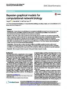
[PDF] Computational Medicine in Data Mining and ... - Google Sites

Special Issue: Computational Intelligence in Data mining ... - CiteSeerX

Editorial Scalable Data Mining Algorithms in Computational ... - Hindawi

Graphical Models for High Dimensional Density Estimation

data mining over graphical results of experiments with domain ...

Data mining techniques for improved WSR-88D rainfall estimation