friends( torn,John). friends( torn,sum). If 1 pose the query ?- party(Name), the above program succeeds with the instantiation Name = sam. Figure 1 shows.
GRAPHICAL DEBUGGING W I T H THE TRANSPARENT PROLOG M A C H I N E (TPM)1 Marc Eisenstadt and Mike Brayshaw Human Cognition Research Laboratory The Open University Milton Keynes MK7 6AA, UK Abstract: An augmented and/or tree representation of logic programs is presented as the basis for an advanced graphical tracing and debugging facility for Prolog. TPM can be run in slow-motion/close-up mode for novices or high-speed/longdistance mode for experts with no attendant conceptual change. Moreover, it deals correctly both with clause head matching and with the cut. The current implementation runs on Apollo workstations, and is written in Prolog. 1
Introduction
In (Eisenstadt, 1985) we developed a model of Prolog execution which gave detailed symptomatic information so that either the programmer could home in directly on trouble spots or else a supervisory program could detect characteristic 'symptom clusters' in order to spot bugs. The current effort is an attempt to provide a significant boost to the practical debugging of very large programs by highly experienced Prolog programmers, while maintaining conceptual clarity for novices. The underlying philosophy of 'retrospective zooming' still applies, but now we include the modern graphical techniques which the earlier work only hinted at. Section 2 describes the underlying principles involved in the design and development of our view of Prolog execution, which we dub The Transparent Prolog Machine' (TPM). Details of the running user environment are presented in section 3, followed by a worked example in section 4. The account which follows assumes that the reader is an experienced Prolog user. 2 TPM: Underlying principles 2.1
AORTA diagrams
An ordinary node in a traditional and/or tree can be enriched to become a full-fledged 'status box' which concisely reveals the execution history of individual clauses. This simple
augmentation, here dubbed the 'AORTA' ('And/OR Tree, Augmented') diagram, is the focal point of our graphical debugger. TPM allows both a long-distance view of execution (displaying several thousand nodes and highlighting 'points of interest' at the user's request) and a close-up view, using all of the detailed notation of AORTA diagrams. To illustrate the close up view, the program below is contrived to use a large number of AORTA diagram features in a small space. party(X):- happy(X), birthday(X). %party if happy & birthday party(X):- friends(X,Y), sad(Y). % or to cheer up sad friend happy(X):- hot, humid, !, swimming(X). happy(X):- cloudy, watchingtv(X). happy(X):- cloudy, having_fun(X). cloudy, humid, hot. having_fun(tom). having_fun(sam). swimming(john). swimming(sam). watching_tv(john). sad(bill). sad(sam). birthday(tom). birthday(sam). friends( torn,John). friends( torn,sum). If 1 pose the query ?- party(Name), the above program succeeds with the instantiation Name = sam. Figure 1 shows the AORTA diagram corresponding to the final snapshot of execution.
Circular nodes are used to depict system primitives (there is one, the cut, in figure 1). The large rectangular boxes in figure 1 are called procedure status boxes. The top half of such boxes shows the status of the goal at the time of viewing. A question mark indicates a pending goal; a tick ('check') indicates a successful goal; a cross indicates a failed goal; a tick/cross combination indicates an initial success followed by subsequent failure on backtracking. The lower half of the procedure status box indicates the number of the latest matching clause head. Thus, in the case of the goal party the tick in the top half of the box indicates that the goal was successful, and the number 2 below it tells us that was the second clause which succeeded. The small vertical lines dangling beneath each procedure status box are known as 'clause branches', and the square boxes at the end of such lines are 'clause status boxes'. Such boxes use the same question-mark, tick, cross, and tick/cross combination to depict the status of individual clauses. If a given clause head does not unify, then a short horizontal 'dead-end' bar is added instead of a clause status box (examples may be seen under the procedure status boxes for sad and birthday in figure 1). Clause branches correspond to 'or' choices, but are drawn differently from their traditional counterparts in order to make the processing of individual clauses obvious at a glance. We use a family metaphor to describe the lineage of goals. In figure 1, happy and birthday are sisters, and their mother is party. Subgoals friends and sad are sisters of one another, but they have a different lineage from that of happy and birthday. We can model this relationship by attributing different paternity to each different clause. In other words, clause heads CI and C2 (labelled purely for the reader's convenience in figure 1) represent different fathers for the different groups of children. Thus, C2 is a step-fat her of birthday, and birthday and friends are step-sisters. To reflect the chronology of execution, we also note that happy is an older sister of birthday, and C2 is & future stepfather of birthday. The family metaphor enables us to provide a concise definition of the behaviour of the cut: it freezes older sister goals and their descendants, eliminates future step-fathers, and then succeeds.
variables; down arrows indicate input variables. Right-angled arrows indicate a variable 'passed across' or shared with a sister goal. Headless arrows indicate directly-matching terms. Often there is a direct visual correspondence between a variable and the arrow showing its instantiation in the diagram (e.g. sam is directly beneath Y3 in its first occurrence next to the status box for friends). Whenever the correspondence is 'indirect', i.e. the instantiation has come 'from elsewhere', we place a small lozenge beneath the variable to show its instantiation at the moment of the AORTA 'snapshot' (e.g. sam is in the lozenge underneath Y3 in its second occurrence next to the status box for sad). Notice in figure 1 that X3 is instantiated to torn, Y3 is instantiated to sam and that this instantiation is passed to the goal sad. The goal sad(Y3), with Y3 instantiated to sam, matches directly against the fact sad(sam) in the database.
Returning to our party example, we can see that happy succeeded initially on clause 1, but unification with either clause of birthday was not possible. This failure caused the backtracking into swim, which itself failed upon backtracking (no further clauses to attempt), as indicated by the tick/cross combination appearing in the top of its status box. This is also the case with the ! goal. Notice the frozen cloud around the cut's older sisters hot and humid and the hashing showing the elimination of the cut's future step-fathers under the procedure status box of the parent goal happy. The parent's failure is further indicated by the tick/cross in the top part of its status box. The failure of clause one of party leads to clause two being attempted. The friends goal succeeds on clause one, i.e. friends(tom, john), but sad(john) fails. This time friends succeeds on the second clause, namely friends (torn, sam), and a brand new invocation of the sad goal occurs. To indicate that there are one or more previous invocations of a goal at the same point in the search space, a dark-shaded ghost status box is drawn. This ghost status box is selectable by the user as a way to observe the state of execution at a particular moment.
The LDV automatically incorporates certain convenient abstractions for simplifying the display. These abstractions are based upon the concept of a shallow cliche, which is a segment of code that can be statically analysed to reveal a characteristic shape or characteristic behaviour. The most prominent shallow cliche, and the only one we deal with at the moment, is tail recursion. The LDV depicts tail recursion by showing only the first two and last two calls, using the equivalent of 'ellipsis dots' in the diagram for all the intervening calls. The intervening call details may be 'opened up' for inspection by the user on request.
To illustrate unification, the relations and arguments next to the top half of each procedure status box depict the state of play when the goal was invoked, whereas the relations and arguments next to the bottom half of each procedure status box depict the matching clause head found in the data base. Userchosen variable names are subscripted automatically to indicate renamed variables. The diagrams use a sideways '=' with arrowheads to show unification. Up arrows indicate output
84
ARCHITECTURES AND LANGUAGES
2.2 LDV: The Long Distance View The long distance view (LDV) is designed to allow the user to retrospectively analyse the global behaviour of very large programs. It shows the execution space of the program (as opposed to the full search space) and the final outcome of attempted goals. This is done by means of a schematized AND/OR tree in which individual nodes summarize the outcome of a call to a particular procedure. Each node is actually a collapsed 'procedure status box', showing just the top half of the procedure status box as introduced above. Powerful gestalt effects are possible even in very long-distance views of large trees, because familiar 'clusters' of nodes are easy to spot, particularly for someone who has been developing the associated code over a period of days, and has become accustomed to the repetition of certain familiar shapes. Potential items of interest can, of course, be inspected more closely, even while preserving a considerable degree of surrounding context. In section 3 we describe our 'selective highlighting' facility which enables the programmer to 'light up' (by blinking or changing the colour of) nodes in the tree which satisfy some particular constraint or behavioural description.
3 A Working Environment 3.1
The Basic Environment
The user environment provides the user with access to the normal Prolog interpreter/compiler via command line input as usual, but extends this by providing menu options to invoke the TPM trace package on a new query or trace a previously executed query. Menu options are also present to support the highlighting and replay options outlined later in this section, as well as to alter the viewport onto, or scale of, the graphics trace in the graphics areas. The area displaying the graphics is mouse sensitive, and clicking on a LDV node produces a 3-ply AORTA diagram with that node at the centre. Ghost status boxes or clause status boxes can also be interrogated via the mouse. The interface provides help documentation for each option associated with a particular mouse button.
3.2
Selective Highlighting
Frequently a user will wish to ask queries of the form 'where did X get instantiated to [a, b]' or 'where in the program does foo get invoked by bar'. To address this problem we provide a Selective Highlighting option in the LDV display. This option allows the user to specify a search 'form' corresponding to the following template: goal: functor arguments parent: functor arguments constraint: term 0 before 0 first 0 success 0 after 0 latest 0 failure For example, we can request the highlighting of all occurrences of the principal functor foo with a second argument instantiated to the list [bar] called by the mother goal gawp. The arguments of gawp need not be specified (even the functor foo need not be specified). The constraint pan of the search form allows us for example to highlight all occurrences of the principal functor foo with a second argument instantiated to some list (indicated by a meta-variable such as L) with the added constraint that the length of L be less man 2. The result of such requests will be for tnTspecified items to be highlighted wherever this combination occurs in the LDV. This facility allows for rapid location and tracing of given functors or variables. It also allows the user to effectively spy a variable or a particular variable instantiation and observe its behaviour retrospectively in the trace. 3.3
Replay
One of the major problems in telling the story of a program's execution is explaining re-instantiation of variables, multiple successes or failures, and other facets of backtracking. We deal with this problem by providing a replay facility whereby the usei can see the dynamic execution of the program through the LDV execution space or AORTA diagrams, clearly indicating failure and subsequent backtracking, re-attempting of goals, subsequent failure, resatisfaction or retries. The replay facility thus allows the user to view the execution space at any given time, or at any particular goal invocation. The user can control the speed of the replay with slow motion and single step options being available. Our replay capability is possible only because we store an exhaustive history of the program's execution. It is our belief that the rewards offered in terms of rapid debugging easily outweigh the overheads of history preservation, particularly in modern (cheap-memory) computing environments. Nontermination however must clearly be avoided e.g. by interpreter stack monitoring a la Shapiro (1983). Just before replay begins (i.e. following a selective highlighting choice or a request to replay from the beginninc), the LDV is 'wound back' to the user-selected point. The interesting thing about the LDV at this point is that it shows a 'pre-ordained' search space, i.e. the LDV shows nodes in the tree which TPM guarantees will eventually form part of the execution space, but which at the moment of replay have yet to be traversed. 3.4
Zooming
Zooming allows the user to see a close up AORTA view of any node chosen from the LDV. Since zooming and highlighting requests always begin with the LDV, all the perspective information associated with the LDV is available at the point of choice, allowing the user clearly to understand the context of the code which is being observed 'close up'. This approach removes the 'forest-vs.-trees' problem associated with
conventional 'spy' packages. In such packages, once a spied' goal is reached it may no longer be clear how you arrived there, how the instantiations of the variables have been derived, what state the program is in, what side-effects have taken place, whether the program has only reached this point on backtracking, and (if a 'redo' is involved) the nature, cause, and scope of the backtracking involved. 4 A Worked Example Consider the following scenario: a pre-stored database describes the contents of a warehouse, giving the reference number, order number, item, price, and quantity, all referenced in terms of the supplier. The database looks like the following: jones(1609,llla,tyres,12.46,30). jacks( 1620,444>Pumps,23.00,15). jacks(1621,477a,wheels,9.99,5). smiths( 1640,370,hubcaps,5.49,43). Now suppose that since the original was drawn up, things like the old reference number, price, and quantity in stock have changed. What we wish now to do is to take items which are currently in stock and check them with the old database, compiling a new database of items and suppliers. If an item is new, i.e. not in the old database, then the program will warn us that a new item is encountered and return the list of known items so far processed. Items that are included in the new database already are ignored. Here is the relevant (buggy) program: search jJb([X|T],[X|Tsl):jones(_,_,X, _,_), store(jones,X), search db(T,Ts). search_db([X|Tl,[X|Ts]):jacks(_,_,X,_,_), store(jacks,X), search_db(T,Ts). search_db([X|T],[X|Ts]):smiths(_,_,Xs,>_,_), store(smiths,Xs), search db(T,Ts). search_db(U,U): nl,write('AH items are known'),nl. search_db(lX|J,n):write('List contains unknown item: '), write(X),nI. store(Manu,Item):manufacturer(Manu,Item). store(ManuJtem):assert(manufacturer(Manu,Item)). Given the query ?- search_db(ltyres,wheels,hubcaps],P). the program appears to be working correctly, and the following new facts are asserted: manufacturer(jones,tyres). manufacturer(jacks,wheels). manufacturer(smiths,hubcaps). Now, if we present it with the query ?- search_db([tyres,wheels,hubcap],P). we expect the program to print out 'List contains unknown item: hubcap', and return with the truncated list P=[tyres,wheels]. Unexpectedly, however, the query succeeds with P=[tyres,wheels,hubcap]. That is, the program claims to know all the items, instead of reporting that it contained an unknown item, namely hubcap. If we ask for an
Eisenatadt and Brayahaw
85
was in error here contained all the variables twice. Indeed the pattern of their occurrence was entirely plausible, since smiths may have used an output variable which was to be dealt with by store if the program semantics were different. Either way the AORTA will show clearly the behaviour of the program. More detailed worked examples, including the replay facility run on a simple compiler, and a discussion of the relationship between TPM and declarative debugging, are presented in (Eisenstadt and Brayshaw, 1987). Figure 2 LDV of ?- search_db(Ityres,wheels,hubcap], P)„ which unexpectedly succeeded. The goal searchdb with first argument (hubcapl 1 is highlighted. LDV of the execution space we will get the diagram depicted in figure 2 (but without the highlighting). Since we are interested in what happened when search db came to deal with hubcap we can use the Selective Highlighting facility to show us where in the tree searchjib gets called with first argument instantiated to [hubcapl ]. Figure 2 shows the result of our highlighting request. Having located this node we can ask TPM to zoom in on the goal. As Figure 3 shows, this gives us a three ply 'AORTA' view of the goal, with the chosen goal in the middle. From the AORTA diagram we can see that its behaviour prior to reaching the chosen goal was entirely as predicted. Once entered it tries to attempt jones(_, ,hubcap v ,_J via clause one and fails. It then attempts to do the same thing, via clause two, for jacks(_,_,hubcap,_,_) with similar results. This is what is expected However we can see at a glance that smiths(_,_,Xs,_,_) succeeds with Xs=hubcaps, the first item in the "database. This is clearly not what was meant to happen! The program should have tried to prove smiths(_,_,hubcap,_, ) but was accidentally called with the uninstanTiated variable Xs as its third argument. This argument subsequently got instantiated by unification with the first fact found for smiths, namely smiths(_,_,hubcaps,__♦__). Note the arrows and lozenges indicating dataflow and variable instantiation in the three selected clauses. This selection was done by the user clicking on a status box leading to the status box 'opening up' to reveal the extra unification information. The correct code for clause 3 of searchdb is shown below: search_db([X|Tl,fX|TsJ):smiths(_,_,X,_, ), store(verb,X), search_db(T,Ts). Given the changed code, the call to smiths will now be smiths(__,__,hubcap,_,_), which will (correctly) fail. TPM helped us to find the bugs within two steps: the LDV highlight and the zoom to the AORTA diagram. Many modern Prolog implementations will find and report as a warning any single occurrences of a variable in a clause. However the clause that
86
ARCHITECTURES AND LANGUAGES
5
Conclusions
Our aim has been to reconcile a global view of Prolog program execution with the 'truth' about unification and clause selection. The key ingredients of our approach have been (i) appreciation of the power of gestalt patterns, (ii) recognition of the need (and the ability) to display thousands of nodes at a time, (iii) enhancement of traditional and/or tree branches with individual clause details, (iv) enhancement of and/or tree nodes with goal 'status boxes' and (v) ability to vary the type of detail being investigated with the particular grain size, rather than using a physical 'zoom'. These ingredients combine to yield an environment which is suitable both for teaching introductory Prolog programming and for assisting the day-to-day efforts of highly experienced Prolog programmers. 6
References
Eisenstadt, M. Retrospective Zooming: a knowledge based tracing and debugging methodology for logic programming. Proceedings of the Ninth International Joint Conference on Artificial Intelligence (IJCAI-85). Los Angeles: Morgan Kaufmann, 1985. Eisenstadt, M., and Brayshaw, M. The Transparent Prolog Machine (TPM): an execution model and graphical debugger for logic programming. Journal ofU)gic Programming, 1987, in press (also available as Technical Report no. 21, Human Cognition Research Laboratory, The Open University, Milton Keynes, 1986.) Shapiro, E. Algorithmic program debugging. Cambridge, Massachussets: MIT Press, 1983.
Figure 3. Zoomed view of the goal search_db(thubciip|_J, as chosen from the LDV.