Graphical Models in Local, Asymmetric Multi-Agent Markov Decision Processes. Dmitri Dolgov and Edmund Durfee. Department of Electrical Engineering and ...
Graphical Models in Local, Asymmetric Multi-Agent Markov Decision Processes Dmitri Dolgov and Edmund Durfee Department of Electrical Engineering and Computer Science University of Michigan Ann Arbor, MI 48109 {ddolgov,durfee}@umich.edu Abstract In multi-agent MDPs, it is generally necessary to consider the joint state space of all agents, making the size of the problem and the solution exponential in the number of agents. However, often interactions between the agents are only local, which suggests a more compact problem representation. We consider a subclass of multi-agent MDPs with local interactions where dependencies between agents are asymmetric, meaning that agents can affect others in a unidirectional manner. This asymmetry, which often occurs in domains with authority-driven relationships between agents, allows us to make better use of the locality of agents’ interactions. We present and analyze a graphical model of such problems and show that, for some classes of problems, it can be exploited to yield significant (sometimes exponential) savings in problem and solution size, as well as in computational efficiency of solution algorithms.
1. Introduction Markov decision processes [9] are widely used for devising optimal control policies for agents in stochastic environments. Moreover, MDPs are also being applied to multiagent domains [1, 10, 11]. However, a weak spot of traditional MDPs that subjects them to “the curse of dimensionality” and presents significant computational challenges is the flat state space model, which enumerates all states the agent can be in. This is especially significant for multi-agent MDPs, where, in general, it is necessary to consider the joint state and action spaces of all agents. Fortunately, there is often a significant amount of structure to MDPs, which can be exploited to devise more compact problem and solution representations, as well as efficient solution methods that take advantage of such representations. For example, a number of factored represenThis work was supported, in part, by a grant from Honeywell Labs.
tations have been proposed [2, 3, 5] that model the state space as being factored into state variables, and use dynamic Bayesian network representations of the transition function to exploit the locality of the relationships between variables. We focus on multi-agent MDPs and on a particular form of problem structure that is due to the locality of interactions between agents. Let us note, however, that we analyze the structure and complexity of optimal solutions only, and the claims do not apply to approximate methods that exploit problem structure (e.g., [5]). Central to our problem representation are dependency graphs that describe the relationships between agents. The idea is very similar to other graphical models, e.g., graphical games [6], coordination graphs [5], and multi-agent influence diagrams [7], where graphs are used to more compactly represent the interactions between agents to avoid the exponential explosion in problem size. Similarly, our representation of a multi-agent MDP is exponential only in the degree of the dependency graph, and can be exponentially smaller than the size of the flat MDP defined on the joint state and action spaces of all agents. We focus on asymmetric dependency graphs, where the influences that agents exert on each other do not have to be mutual. Such interactions are characteristic of domains with authority-based relationships between agents, i.e. lowauthority agents have no control over higher-authority ones. Given the compact representation of multi-agent MDPs, an important question is whether the compactness of problem representation can be maintained in the solutions, and if so, whether it can be exploited to devise more efficient solution methods. We analyze the effects of optimization criteria and shape of dependency graphs on the structure of optimal policies, and for problems where the compactness can be maintained in the solution, we present algorithms that make use of the graphical representation.
2. Preliminaries In this section, we briefly review some background and introduce our compact representation of multi-agent MDPs.
2.1. Markov Decision Processes A single-agent MDP can be defined as a n-tuple hS, A, P, Ri, where S = {i} and A = {a} are finite sets of states and actions, P : S × A × S → [0, 1] defines the transition function (the probability that the agent goes to state j if it executes action a in state i is P (i, a, j)), and R : S → R defines the rewards (the agent gets a reward of R(i) for visiting state i).1 A solution to a MDP is a policy defined as a procedure for selecting an action. It is known [9] that, for such MDPs, there always exist policies that are uniformly-optimal (optimal for all initial conditions), stationary (time independent), deterministic (always select the same action for a given state), and Markov (history-independent); such policies (π) can be described as mappings of states to actions: π : S → A. Let us now consider a multi-agent environment with a set of n agents M = {m} (|M| = n), each of whom has its own set of states Sm = {im } and actions Am = {am }. The most straightforward and also the most general way to extend the concept of a single-agent MDP to the fullyobservable multi-agent case is to assume that all agents affect the transitions and rewards of all other agents. Under these conditions, a multi-agent MDP can be defined simply as a large MDP hSM , AM , PM , RM i, where the joint state space SM is defined as the cross product of the state spaces of all agents: SM = S1 × . . . × Sn , and the joint action space is the cross product of the action spaces of all agents: AM = A1 × . . . × An . The transition and the reward functions are defined on the joint state and action spaces of all agents in the standard way: PM : SM ×AM ×SM → [0, 1] and RM : SM → R. This representation, which we refer to as flat, is the most general one, in that, by considering the joint state and action spaces, it allows for arbitrary interactions between agents. The trouble is that the problem (and solution) size grows exponentially with the number of agents. Thus, very quickly it becomes impossible to even write down the problem, let alone solve it. Let us note that, if the state space of each agent is defined on a set of world features, there can be some overlap in features between the agents, in which case the joint state space would be smaller than the cross product of the state space of all agents, and would grow as a slower exponent. For simplicity, we ignore the possibility of overlapping features, but our results are directly applicable to that case as well.
2.2. Graphical Multi-Agent MDPs In many multi-agent domains, the interactions between agents are only local, meaning that the rewards and tran1
Often, rewards are said to also depend on actions and future states. For simplicity, we define rewards as function of current state only, but our model can be generalized to the more general case.
1
2
1
1
4
2
2
(b)
(c)
m 3
(a)
Figure 1. Agent Dependency Graphs
sitions of an agent are not directly influenced by all other agents, but rather only by a small subset of them. To exploit the sparseness in agents’ interactions, we propose a compact representation that is analogous to the Bayesian network representation of joint probability distributions of several random variables. Given its similarity to other graphical models, we label our representation a graphical multi-agent MDP (graphical MMDP). Central to the definition of a graphical MMDP is a notion of a dependency graph (Figure 1), which shows how agents affect each other. The graph has a vertex for every agent in the multi-agent MDP. There is a directed edge from vertex k to vertex m if agent k has an influence on agent m. The concept is very similar to coordination graphs [5], but we distinguish between two ways agents can influence each other: (1) an agent can affect another agent’s transitions, in which case we use a solid arrow to depict this relationship in the dependency graph, and (2) an agent can affect another agent’s rewards, in which case we use a dashed arrow in the dependency graph. To simplify the following discussion of graphical multiagent MDPs, we also introduce some additional concepts and notation pertaining to the structure of the dependency graph. For every agent m ∈ M, let us label all agents − (P ) (parents of m that directly affect m’s transitions as Nm with respect to transition function P ), and all agents whose + transitions are directly affected by m as Nm (P ) (children of m with respect to transition function P ). Similarly, we − (R) to refer to agents that directly affect m’s reuse Nm + (R) to refer to agents whose rewards are diwards, and Nm rectly affected by m. Thus, in the graph shown in Figure − − + 1a, Nm (P ) = {1, 4}, Nm (R) = {1, 2}, Nm (P ) = {3}, + and Nm (R) = {4}. We use the terms “transition-related” and “reward-related” parents and children to distinguish between the two categories. Sometimes, it will also be helpful to talk about the union of transition-related and reward− related parents in which case use Nm = S − or children, S we − + + + Nm (P ) Nm (R) and Nm = Nm (P ) Nm (R). Furthermore, let us label the set of all ancestors of m (all agents from which m is reachable) with respect to transition− related and reward-related dependencies as Om (P ) and − Om (R), respectively. Similarly, let us label the descendants + + of m (all agents reachable from m) as Om (P ) and Om (R). A graphical MMDP with a set of agents M is defined as follows. Associated with each agent m ∈ M is a n-tuple
hSm , Am , Pm , Rm i, where the state space Sm and the action space Am are defined exactly as before, but the transition and the reward functions are defined as follows: − Pm : SNm (P ) × Sm × Am × Sm → [0, 1] − Rm : SNm (R) × Sm → R,
(1)
− − where SNm (P ) and SNm (R) are the joint state spaces of the transition-related and reward-related parents of m, respectively. In other words, the transition function of agent m specifies a probability distribution over its next states Sm as a function of its own current state Sm and the current − states of its parents SNm (P ) and its own action Am . That is − P (iNm (P ) , im , am , jm ) is the probability that agent m goes to state jm if it executes action am when its current state is − im and the states of its transition-related parents are iNm (P ) . The reward function is defined analogously on the current states of the agent itself and the reward-related parents. Also notice that we allow cycles in the agent dependency graph, and moreover the same agent can both influence and be influenced by some other agent (e.g. agents 4 and m in Figure 1a). We also allow for asymmetric influences between agents, i.e. it could be the case that one agent affects the other, but not vice versa (e.g. agent m, in Figure 1a, is influenced by agent 1, but the opposite is not true). This is often the case in domains where the relationships between agents are authority-based. It turns out that the existence of such asymmetry has important implications on the compactness of the solution and the complexity of the solution algorithms. We return to a discussion of the consequences of this asymmetry in the following sections. It is important to note that, in this representation, each transition and reward function only specifies the rewards and transition probabilities of agent m, and contains no information about the rewards and transitions of other agents. This implies that the reward and next state of agent m are conditionally independent of the rewards and the next states of other agents, given the current action of m and the state − of m and its parents Nm . Therefore, this model does not allow for correlations between the rewards or the next states of different agents. For example, we cannot model the situation where two agents are trying to go through the same door and whether one agent makes it depends on whether the other one does; we can only represent, for each agent, the probability that it makes it, independently of the other. This limitation of the model can be overcome by “lumping together” groups of agents that are correlated in such ways into a single agent as in the flat multi-agent MDP formulation. In fact, we could have allowed for such dependencies in our model, but it would have complicated the presentation. Instead, we assume that all such correlations have already been dealt with, and the resulting problem only consists of agents (perhaps composite ones) whose states and rewards have this conditional independence property.
It is easy to see that the size of a problem represented in this fashion is exponential in the maximum number of parents of any agent, but unlike the flat model, it does not depend on the total number of agents. Therefore, for problems where agents have a small number of parents, space savings can be significant. In particular, if the number of parents of any agent is bounded by a constant, the savings are exponential (in terms of the number of agents).
3. Properties of Graphical Multi-Agent MDPs Now that we have a compact representation of multiagent MDPs, two important questions arise. First, can we compactly represent the solutions to these problems? And second, if so, can we exploit the compact representations of the problems and the solutions to improve the efficiency of the solution algorithms? Positive answers to these questions would be important indications of the value of our graphical problem representation. However, before we attempt to answer these questions and get into a more detailed analysis of the related issues, let us lay down some groundwork that will simplify the following discussion. First of all, let us note that a graphical multi-agent MDP is just a compact representation, and any graphical MMDP can be easily converted to a flat multi-agent MDP, analogously to how a compact Bayesian network can be converted to a joint probability distribution. Therefore, all properties of solutions to flat multi-agent MDPs (e.g. stationarity, history-independence, etc.) also hold for equivalent problems that are formulated as graphical MMDPs. Thus, the following simple observation about the form of policies in graphical MMDPs holds. Observation 1 For a graphical MMDP hSm , Am , Pm , Rm i, m ∈ M, with an optimization criterion for which optimal policies are Markov, stationary, and deterministic,2 such policies can be represented as πm : SXm → Am , where SXm is a cross product of the state spaces of some subset of all agents (Xm ⊆ M). Clearly, this observation does not say much about the compactness of policies, since it allows Xm = M, which corresponds to a solution where an agent has to consider the states of all other agents when deciding on an action. If that were always the case, using this compact graphical representation for the problem would not (by itself) be beneficial, because the solution would not retain the compactness and would be exponential in the number of agents. However, as it turns out, for some problems, Xm can be significantly smaller than M. Thus we are interested in determining, for every agent m, the minimal set of agents whose states m’s policy has to depend on: 2
We will implicitly assume that optimal policies are Markov, stationary, and deterministic from now on.
Definition 1 In a graphical MMDP, a set of agents Xm is a minimal domain of an optimal policy πm : SXm → Am 0 of agent m iff, for any set of agents Y and any policy πm : SY → Am , the following implications hold: 0 Y ⊂ Xm =⇒ U (πm ) < U (πm ) 0 Y ⊇ Xm =⇒ U (πm ) ≤ U (πm ),
where U (π) is the payoff that is being maximized. Essentially, this definition allows us to talk about the sets of agents whose joint state space is necessary and sufficient for determining optimal actions of agent m. From now on, whenever we use the notation πm : SXm → Am , we implicitly assume that Xm is the minimal domain of πm .
3.1. Assumptions As mentioned earlier, one of the main goals of the following sections will be to characterize the minimal domains of agents’ policies under various conditions. Let us make a few observations and assumptions about properties of minimal domains that allow us to avoid some non-interesting degenerate special cases and to focus on the “hardest” cases in our analysis. These assumptions do not limit the general complexity results that follow, as the latter only require that there exist some problems for which the assumptions hold. In the rest of the paper, we implicitly assume that they hold. Central to our future discussion will be an analysis of which random variables (rewards, states, etc.) depend on which others. It will be very useful to talk about the conditional independence of future values of some variables, given the current values of others. Definition 2 We say that a random variable X is Markov on the joint state space SY of some set of agents Y if, given the current values of all states in SY , the future values of X are independent of any past information. If that property does not hold, we say that X is non-Markov on SY . Assumption 1 For a minimal domain Xm of agent m’s optimal policy, and a set of agents Y, the following hold: 1. Xm is unique 2. m ∈ Xm 3. l ∈ Xm =⇒ Sl is Markov on SXm 4. Sm is Markov on SY ⇐⇒ Y ⊇ Xm The first assumption allows us to avoid some special cases with sets of agents with highly-correlated states, where equivalent policies can be constructed as functions of either of the sets. The second assumption implies that an optimal policy of every agent depends on its own state. The third assumption says that the state space of any agent l that is in the minimal domain of m must be Markov on the state space of the minimal domain. Since the state space of agent
l is in the minimal domain of m, it must influence m’s rewards in a non-trivial manner. Thus, if Sl is non-Markov on SXm , agent m should be able to expand the domain of its policy to make Sl Markov, since that, in general, would increase m’s payoff. The fourth assumption says that the agent’s state is Markov only on supersets of its minimal domain, because the agent would want to increase the domain of its policy just enough to make its state Markov. These assumptions are slightly redundant (e.g., 4 could be deduced from weaker conditions), but we use this form for brevity.
3.2. Transitivity Using the results of the previous sections, we can now formulate an important claim that will significantly simplify the analysis that follows. Proposition 1 Consider two agents m, l ∈ M, where the optimal policies of m and l have minimal domains of Xm and Xl , respectively (πm : SXm → Am , πl : SXl → Al ). Then, under Assumption 1, the following holds: l ∈ Xm =⇒ Xl ⊆ Xm , Proof: We will show this by contradiction. Let us consider an agent from l’s minimal domain: k ∈ Xl . Let us assume (contradicting the statement of the proposition) that l ∈ Xm , but k ∈ / Xm . Consider the set of agents that consists of the union of the two minimalSdomains Xm and Xl , but with agent k removed: Ym = Xm (Xl \k). Then, since Ym + Xl , Assumption 1.4 implies that Sl is non-Markov on SYm . Thus, Assumption 1.3 implies l ∈ / Xm , which contradicts our earlier assumption. � Essentially, this proposition says that the minimal domains have a certain “transitive” property: if agent m needs to base its action choices on the state of agent l, then, in general, m also needs to base its actions on the states of all agents in the minimal domain of l. As such, this proposition will help us to establish lower bounds on policy sizes. In the rest of the paper, we analyze some classes of problems to see how large the minimal domains are, under various conditions and assumptions, and for domains where minimal domains are not prohibitively large, we outline solution algorithms that exploit graphical structure. In what follows, we focus on two common scenarios: one, where the agents work as a team and aim to maximize the social welfare of the group (sum of individual payoffs), and the other, where each agent maximizes its own payoff.
4. Maximizing Social Welfare The following proposition characterizes the structure of the optimal solutions to graphical multi-agent MDPs under the social welfare optimization criterion, and as such serves
as an indication of whether the compactness of this particular representation can be exploited to devise an efficient solution algorithm for such problems. We demonstrate that, in general, when the social welfare of the group is considered, the optimal actions of each agent depend on the states of all other agents (unless the dependency graph is disconnected). Let us note that this case where all agents are maximizing the same objective function is equivalent to a singleagent factored MDP, and our results for this case are analogous to the well-known fact that the value function in a single-agent factored MDP does not, in general, retain the structure of the problem [8]. Proposition 2 For a graphical MMDP with a connected (ignoring edge directionality) dependency graph, under the optimization criterion that maximizes the social welfare of all agents, an optimal policy πm of agent m, in general, depends on the states of all other agents, i.e. πm : SM → Am . Proof (Sketch): Agent m must, at the minimum, base its action decisions on the states of its immediate (both transitionand reward-related) parents and children. Indeed, agent m should worry about the states of its transition-related par− ents, Nm (P ), because their states affect the one-step transition probabilities of m, which certainly have a bearing on m’s payoff. Agent m should also include in the domain of − (R), its policy the states of its reward-related parents, Nm because they affect m’s immediate rewards and agent m might need to act so as to “synchronize” its state with the state of its parents. Similarly, since the agent cares about the social welfare of all agents, it will need to consider the effect that its actions have on the states and rewards of its immediate children, and must thus base its policy on the states + + (R) to potentially (P ) and Nm of its immediate children Nm “set them up” to get higher rewards. Having established that the minimal domain of each agent must include the immediate children and parents of the agent, we can use the transitivity property from the previous section to extend this result. Although Proposition 1 only holds under the conditions of Assumption 1, for our purpose of determining the complexity of policies in general, it is sufficient that there exist problems for which Assumption 1 holds. It follows from Proposition 1 that the minimal domain of agent m must include all parents and children of m’s parents and children, and so forth. For a connected dependency graph, this expands the minimal domain of each agent to all other agents in M. � The above result should not be too surprising, as it makes clear, intuitive sense. Indeed, let us consider a simple example that has a flavor of a commonly-occurring production scenario. Suppose that there is a set of agents that can either cooperate to generate a certain product, yielding a very high reward, or they can concentrate on some local tasks that do not require cooperation, but which have lower so-
cial payoff. Also, suppose that the interactions between the agents are only local – for example, the agents are operating an assembly line, where each agent receives the product from a previous agent, modifies it, and passes it on to the next agent. Let us now suppose that each agent has a certain probability of breaking down, and if that happens to at least one of the agents, the assembly line fails. In such an example, the optimal policy for the agents would be to participate in the assembly-line production until one of them fails, at which point all agents should switch to working on their local tasks (perhaps processing items already in the pipeline). Clearly, in that example, the policy of each agent is a function of the states of all other agents. The take-home message of the above is that, when the agents care about the social welfare of the group, even when the interactions between the agents are only local, the agents’ policies depend on the joint state space of all agents. The reason for this is that a state change of one agent might lead all other agents to want to immediately modify their behavior. Therefore, our particular type of compact graphical representation (by itself and without additional restrictions) cannot be used to compactly represent the solutions.
5. Maximizing Own Welfare In this section, we analyze problems where each of the agents maximizes its own payoff. Under this assumption, unlike the discouraging scenario of the previous section, the complexity of agents’ policies is slightly less frightening. The following result characterizes the size of the minimal domain of optimal policies for problems where each agent maximizes its own utility. Proposition 3 For a graphical MMDP with an optimization criterion where each agent maximizes its own reward, the minimal domain of m’s policy consists of m itself and all − , of its transition- and reward-related ancestors: Xm = Em S − S − − where we define Em = m Om (P ) Om (R). Proof (Sketch): To show the correctness of the proposition, we need to prove that, (1) the minimal domain must include − at least m itself and its ancestors (Xm ⊇ Em ), and (2) that − Xm does not include any other agents (Xm ⊆ Em ). We can show (1) by once again applying the transitivity property. Clearly, an agent’s policy should be a function of the states of the agent’s reward-related and transitionrelated parents, because they affect the one-step transition probabilities and rewards of the agent. Then, by Proposition 1, the minimal domain of the agent’s policy must also include all of its ancestors. We establish (2) as follows. We assume that it holds for all ancestors of m, and show that it must then hold for m. We then expand the statement to all agents by induction.
Let us fix the policies πk of all agents except m. Consider e −, R e − i, where Pe − and R e − are − , Am , P the n-tuple hSEm Em Em Em Em defined as follows: − − (i − , am , j − ) = Pm (i , im , am , jm ) PeEm Em Em � Nm (P ) � Y Pk iN − (P ) , ik , πk (iE − ), jk k
k
− k∈Om
(2)
e − (i − ) = Rm (i − , im ) R E m Em Nm (R) − and The above constitutes a fully-observable MDP on SEm em . Am with transition function Pem and reward function R Let us label this decision process M DP1 . By properties of fully-observable MDPs, there exists an optimal stationary 1 1 − → Am . : SEm deterministic solution πm of the form πm Also consider the following MDP on an augmented state space that includes the joint state space of all the agents (and bM i, not just m’s ancestors): M DP2 = hSM , Am , PbM , R b b where PM and RM are defined as follows: − PbM (iM , am , jM ) = Pm (iNm (P ) , im , am , jm ) � � Y Pk iN − (P ) , ik , πk (iE − ), jk k
k
− k∈Om
Y
� � Pk iN − (P ) , ik , πk (iM ), jk
(3)
k
− k∈M\m\Om
bM (iM ) = Rm (i − , im ) R Nm (R) Basically, we have now constructed two fully-observable − , and M DP2 that MDPs: M DP1 that is defined on SEm is defined on SM , where M DP1 is essentially a “projec− . We need to show that no sotion” of M DP2 onto SEm lution to M DP2 can have a higher value3 than the optimal solution to M DP1 . Let us refer to the optimal solu1 2 tion to M DP1 as πm . Suppose there exists a solution πm to 1 2 M DP2 that has a higher value than πm . The policy πm defines some stochastic trajectory for the system over the state space SM . Let us label the distribution over the state space at time t as ρ(iM , t). It can be shown that under our assumptions we can always construct a non-stationary policy 1 − → Am for M DP1 that yields the same disπ em (t) : SEm − as the one protribution ρ(iM , t) over the state space SEm 2 duced by πm . Thus, there exists a non-stationary solution to 1 M DP1 that has a higher payoff than πm , which is a contra1 diction, since we assumed that πm was optimal for M DP1 . We have therefore shown that, given that the policies of all ancestors of m depend only on their own states and the states of their ancestors, there always exists a policy that − ) to m’s maps the state space of m and its ancestors (SEm actions (Am ) that is at least as good as any policy that maps 3
The proof does not rely on the actual type of optimization criterion used by each agent and holds for any criterion that is a function only of the agents’ trajectories.
the joint space of all agents (SM ) to m’s actions. Then, by using induction, we can expand this statement to all agents (for acyclic graphs we use the root nodes as the base case, and for cyclic graphs, we use agents that do not have any ancestors that are not simultaneously their descendants). � The point of the above proposition is that, for situations where each agent maximizes its own utility, the optimal actions of each agent do not have to depend on the states of all other agents, but rather only on its own state and the states of its ancestors. In contrast to the conclusions of Section 4, this result is more encouraging. For example, for dependency graphs that are trees (typical of authority-driven organizational structures), the number of ancestors of any agent equals the depth of the tree, which is logarithmic in the number of agents. Therefore, if each agent maximizes its own welfare, the size of its policy will be exponential in the depth of the tree, but only linear in the number of agents.
5.1. Acyclic Dependency Graphs Thus far we have shown that problems where agents optimize their own welfare can allow for more compact policy representations. We now describe an algorithm that exploits the compactness of the problem representation to more efficiently solve such policy optimization problems for domains with acyclic dependency graphs. It is a distributed algorithm where the agents exchange information, and each one solves its own policy optimization problem. The algorithm is very straightforward and works as follows. First, the root nodes of the graph (the ones with no parents) compute their optimal policies that are simply mappings of their own states to their own actions. Once a root agent computes a policy that maximizes its welfare, it sends the policy to all of its children. Each child waits to − receive the policies πk , k ∈ Nm from its ancestors, then forms a MDP on the state space of itself and its ancestors as e −, R e −i − , Am , P in (eq. 2). It then solves this MDP hSEm Em Em − to produce a policy πm : Em → Am , at which point it sends the policy and the policies of its ancestors to its children. The process repeats until all agents compute their optimal policies. Essentially, this algorithm performs, in a distributed manner, a topological sort of the dependency graph, and computes a policy for every agent.
5.2. Cyclic Dependency Graphs We now turn our attention to the case of dependency graphs with cycles. Note that the complexity result of Proposition 3 still applies, because no assumptions about the cyclic or acyclic nature of dependency graphs were made in the statement or proof of the proposition. Thus, the minimal domain of an agent’s policy is still the set of its ancestors.
The problem is, however, that the solution algorithm of the previous section is inappropriate for cyclic graphs, because it will deadlock on agents that are part of a cycle, since these agents will be waiting to receive policies from each other. Indeed, when self-interested agents mutually affect each other, it is not clear how they should go about constructing their policies. Moreover, in general, for such agents there might not even exist a set of stationary deterministic policies that are in equilibrium, i.e., since the agents mutually affect each other, the best responses of agents to each others’ policies might not be in equilibrium. A careful analysis of this case falls in the realm of Markov games, and is beyond the scope of this paper. However, if we assume that there exists an equilibrium in stationary deterministic policies, and that the agents in a cycle have some “black-box” way of constructing their policies, we can formulate an algorithm for computing optimal policies, by modifying the algorithm from the previous section as follows. The agents begin by finding the largest cycle they are a part of, and then, after the agents receive policies from their parents who are not also their descendants, the agents proceed to devise an optimal joint policy for their cycle, which they then pass to their children.
6. Additive Rewards In our earlier analysis, a reward function Rm of an agent could depend in an arbitrary way on the current states of the agent and its parents (eq. 1). In fact, this is why agents, in general, needed to “synchronize” their states with the states of their parents (and children in the social welfare case), which, in turn, was why the effects of reward-related dependencies propagated just as the transition-related ones did. In this section, we consider a subclass of reward functions whose effects remain local. Namely, we focus on additively-separable reward functions: X − Rm (iNm rmk (ik ), (4) (R) , im ) = rmm (im ) + − k∈Nm (R)
where rmk is a function (rmk : Sk → R) that specifies the contribution of agent k to m’s reward. In order for all of our following results to hold, these functions have to be subject to the following condition: rmk (ik ) = lmk (rkk (ik )),
(5)
where lmk is a positive linear function (lmk (x) = αx + β, α > 0, β ≥ 0). This condition implies that agents’ preferences over each other states are positively (and linearly) correlated, i.e., when an agent increases its local reward, its contribution to the rewards of its reward-related children also increases linearly. Furthermore, the results of this section are only valid under certain assumptions about the optimization criteria the
agents use. Let us say that if an agent receives a history of rewards H(r) = {r(t)} = {r(0), r(1), . . .}, its payoff is � U (H(r)) = U r(0), r(1), . . . . Then, in order for our results to hold, U has to be linear additive: U (H(r1 + r2 )) = U (H(r1 )) + U (H(r2 ))
(6)
Notice that this assumption holds for the commonly-used risk-neutral MDP optimization criteria, such as expected total reward, expected total discounted reward, and average per-step reward, and is, therefore, not greatly limiting. In the rest of this section, for simplicity, we focus on problems with two agents – more specifically, on two interesting special cases, shown in Figure 1b and 1c. However, the results can be generalized to problems with multiple agents and arbitrary dependency graphs. First of all, let us note that both of these problems have cyclic dependency graphs. Therefore, if the reward functions of the agents were not additively-separable, per our earlier results of Section 5, there would be no guarantee that there exists an equilibrium in stationary deterministic policies. However, as we show below, our assumption about the additivity of the reward functions changes that and ensures that an equilibrium always exists. Let us consider the case in Figure 1b. Clearly, the policy of neither agent affects the transition function of the other. Thus, given our assumptions about additivity of rewards and utility functions, it is easy to see that the problem of maximizing the payoff is separable for each agent. For example, for agent 1 we have: � � max U1 H(R1 ) = max U1 H(r11 + r21 ) = π1 ,π2 π1 ,π2 � � (7) max U H(r11 ) + max U H(r21 ) π1
π2
Thus, regardless of what policy agent 2 chooses, agent 1 should adopt a policy that maximizes the first term in (eq. 7). In game-theoretic terms, each of the agents has a (weakly) dominant strategy, and will adopt that strategy, regardless of what the other agent does. This is what guarantees the above-mentioned equilibrium. Also notice that this result does not rely on reward linearity (eq. 5) and holds for any additively-separable (eq. 4) reward functions. Now that we have demonstrated that, for each agent, it suffices to optimize a function of only that agent’s own states and actions, it is clear that each agent can construct its optimal policy independently. Indeed, each agent has to solve a standard MDP on its own state and action space with 0 a slightly modified reward function: Rm (im ) = rmm (im ), which differs from the original reward function (eq. 4) in that it ignores the contribution of m’s parents to its reward. Let us now analyze the case in Figure 1c, where the state of agent 1 affects the transition probabilities of agent 2, and the state of agent 2 affects the rewards of agent 1. Again,
without the assumption that rewards are additive, this cycle would have caused the policies of both agents to depend on the cross product of their state spaces S1 × S2 , and furthermore the existence of equilibria in stationary deterministic policies between self-interested agents is not guaranteed. However, when rewards are additive, the problem is simpler. Indeed, due to our additivity assumptions, we can write the optimization problems of the two agents as: max U1 (. . .) = max U1 (H(r11 )) + max U1 (H(r12 ))
π1 ,π2
π1
π1 ,π2
max U2 (. . .) = max U2 (H(r21 )) + max U2 (H(r22 ))
π1 ,π2
π1
π1 ,π2
(8) Notice that here the problems are no longer separable (as in the previous case), so neither agent is guaranteed to have a dominant strategy. However, if we make use of the assumption that the rewards are positively and linearly correlated (eq. 5), we can show that there always exists an equilibrium in stationary deterministic policies. This is due to the fact that a positive linear transformation of the reward function does not change the optimal policy (we show this for discounted MDPs, but the statement holds more generally): Observation 2 Consider two MDPs: Λ = hS, A, R, P i and Λ0 = hS, A, R0 , P i, where R0 (s) = α(R(s)) + β, α > 0 and β ≥ 0. Then, a policy π is optimal for Λ under the total expected discounted reward optimization criterion iff it is optimal for Λ0 . Proof (Sketch): It is easy to see that the linear transformation R0 (i) = αR(i) + β of the reward function will lead to a linear transformation of the Q function: Q0 (i, a) = αQ(i, a) + β(1 − γ)−1 , where γ is the discount factor. Indeed, the multiplicative factor α just changes the scale of all rewards, and the additive factor β simply produces an extra discounted sequence of rewards that sums to β(1 − γ)−1 over an infinite horizon. Then, since the optimal policy is π(i) = maxa αQ(i, a) + β(1 − γ)−1 = maxa Q(i, a), a policy π is optimal for Λ iff it is optimal for Λ0 . � Observation 2 implies that, for any policy π1 , a policy π2 that maximizes the second term of U1 in (eq. 8) will be simultaneously maximizing (given π1 ) the second term of U2 in (eq. 8). In other words, given any π1 , both agents will agree on the choice of π2 . Therefore, agent 1 can find the pair hπ1 , π2 i that maximizes its payoff U1 and adopt that π1 . Then, agent 2 will adopt the corresponding π2 , since deviating from it cannot increase its utility. To sum up, when rewards are additively-separable (eq. 4) and satisfy (eq. 5), for the purposes of determining the minimal domain of agents’ policies (in two-agent problems), we can ignore reward-related edges in dependency graphs. Furthermore, for graphs where there are no cycles with transition-related edges, the agents can formulate their optimal policies via algorithms similar to the ones described in Section 5.1, and these policies will be in equilibrium.
7. Conclusions We have analyzed the use of a particular compact, graphical representation for a class of multi-agent MDPs with local, asymmetric influences between agents. We have shown that, generally, because the effects of these influences propagate with time, the compactness of the representation is not fully preserved in the solution. We have shown this for multi-agent problems with the social welfare optimization criterion, which are equivalent to single-agent problems, and for which similar results are known. We have also analyzed problems with self-interested agents, and have shown the complexity of solutions to be less prohibitive in some cases (acyclic dependency graphs). We have demonstrated that under further restrictions on agents’ effects on each other (positive-linear, additively-separable rewards), locality is preserved to a greater extent – equilibrium sets of stationary deterministic policies for self-interested agents always exist even in some classes of problems with rewardrelated cyclic relationships between agents. Our future work will combine the graphical representation of multi-agent MDPs with other forms of problem factorization, including constrained multi-agent MDPs [4].
References [1] C. Boutilier. Sequential optimality and coordination in multiagent systems. In IJCAI-99, pages 478–485, 1999. [2] C. Boutilier, T. Dean, and S. Hanks. Decision-theoretic planning: Structural assumptions and computational leverage. JAIR, 11:1–94, 1999. [3] C. Boutilier, R. Dearden, and M. Goldszmidt. Stochastic dynamic programming with factored representations. Artificial Intelligence, 121(1-2):49–107, 2000. [4] D. A. Dolgov and E. H. Durfee. Optimal resource allocation and policy formulation in loosely-coupled Markov decision processes. In ICAPS-04, 2004. To Appear. [5] C. Guestrin, D. Koller, R. Parr, and S. Venkataraman. Efficient solution algorithms for factored MDPs. Journal of Artificial Intelligence Research, 19:399–468, 2003. [6] M. Kearns, M. L. Littman, and S. Singh. Graphical models for game theory. In Proc. of UAI01, pages 253–260, 2001. [7] D. Koller and B. Milch. Multi-agent influence diagrams for representing and solving games. In IJCAI-01, pages 1027– 1036, 2001. [8] D. Koller and R. Parr. Computing factored value functions for policies in structured MDPs. In IJCAI-99, pages 1332– 1339, 1999. [9] M. L. Puterman. Markov Decision Processes. John Wiley & Sons, New York, 1994. [10] D. Pynadath and M. Tambe. Multiagent teamwork: Analyzing the optimality and complexity of key theories and models. In AAMAS-02, 2002. [11] S. Singh and D. Cohn. How to dynamically merge Markov decision processes. In M. I. Jordan, M. J. Kearns, and S. A. Solla, editors, NIPS-98, volume 10. The MIT Press, 1998.