ing a development of model parameter spaces. ... plex systems simulations code development. ... running on desktop PCs; Apple iPad and Samsung Galaxy.
Graphics on Web Platforms for Complex Systems Modelling and Simulation T.H. McMullen, K.A. Hawick, V. Du Preez and B. Pearce Computer Science, Institute for Information and Mathematical Sciences, Massey University, North Shore 102-904, Auckland, New Zealand {t.h.mcmullen, k.a.hawick}@massey.ac.nz, {dupreezvictor, brad.pearce.nz}@gmail.com Tel: +64 9 414 0800 Fax: +64 9 441 8181 April 2012 ABSTRACT Graphical interactive simulations are a powerful means of exploring properties of complex systems models and aiding a development of model parameter spaces. Platform independence for graphics intensive simulations – and especially those involving 3D rendering – has been a difficult goal to realise until recently. We describe use of WebGL, JavaScript and associated graphics rendering interfaces to implement a range of complex system simulations for a Web platform. We experimented with various shading and rendering approaches. We compare the performance obtained using this approach for various compute devices. We discuss performance and implementation issues and the implications for future platform independence of complex systems simulations code development. KEY WORDS WebGL; JavaScript; portable shading; platform independent graphics
1
Introduction
Interactive graphical rendering is an important tool in exploring the parameter space of complex system simulations. Such simulations include models in physics, chemistry, biology, sociology and finance. All these areas have in common a need to adjust the parameters in a model to develop an intuition and understanding of what they mean and how they affect system behaviour [5]. Platform independent computing is a desirable goal for many software projects. Much work has been done using virtual machines and related approaches to platform independence [1]. The advent of widely available tablet computers has renewed interest in platform independence, particularly for high quality graphical rendering programs that can run with a (portable) web browser environment on a range of platforms. Such devices open up a range of potential applications that can use interactive graphics [12, 16].
New and emergent approaches to user interface design for such devices are also an exciting arena for interactive simulations [11]. Computational steering is the term introduced by both Smarr [14] and Fox [3], to describe the interactive exploration of parameter space – often prior to launching a series of non-interactive compute jobs to gather statistics from numerical experiments. The early stages of interacting with the parameter space can save a great deal of time and computational effort by identifying where to look and where to direct study. High performance graphics is a huge aid to computational steering. High quality rendering of a complex system greatly aids in understanding the model. Graphical rendering of complex systems - particularly in 3D involves non-trivial amounts of computation however. Until relatively recently it has really only been practical to work with a high performance graphical rendering or shading system such as OpenGL or its proprietary equivalent. Although such code can sometimes be ported – with a greater or lesser ease depending upon the system involved – to different hardware and operating systems platforms, it has been difficult to realise the goal of complete platform independence. Most recent work has focused on development of custom “Apps” for individual tablets or mobile phones [2]. Tools such as WebGL, JavaScript and associated software systems do open up a practical possibility of developing high graphical quality and reasonably high performance interactive rendering simulations that can be run through a web browser. This is obviously attractive since these will be supported on any platform that supports the appropriate web browser standard. In this paper we develop a set of six computational simulation models that also have significant graphical rendering requirements. We implement these models using platform independent software technologies and investigate
their relative performance on web browser environments running on desktop PCs; Apple iPad and Samsung Galaxy tablet devices. Our article is structured as follows: In Section 2 we describe some of the typical graphical simulation models that we might wish to port to run on various platforms and relate their key features. In Section 3 we present details of our implementation experiments. We present some graphical and performance results in Section 4 and a discussion of their implications in Section 5 in which we also we summarise our findings and give some areas for future work.
2
Simulation Models
We summarise the main features of the simulation models we deployed, giving references where more details can be obtained. Several models were used to test web platforms as a method for modeling complex systems and simulations. Firstly several 2D models were created, including Conway’s Game of Life [4], Diffusion Limited Aggregation (DLA) [18], and an Ising model [9, 10] among others. These 2D models shared similar behaviour, and as such the methods for one can be used across a range of them. To test the use of 3D graphics on a web platform a 3D Ising model was constructed, with two different implementations. These have similar methods for the creation and manipulation of the simulation, but differ in how it is displayed. The first model implemented was Conway’s Game of Life. This was as it is simple to implement with a well defined rule set. To start with two 2D lattices are created, and one initialized with a random or predefined state. From this state the program will work through that lattice and write the updated value for each cell onto the other lattice. The rules for updating a location on the lattice is that so the program will look at the eight closest neighbors, and count the number which are alive. Based on the amount of alive neighbors the cell will become dead or alive or stay in its current state. This state is represented by the colour of the cell, with white been dead while red if alive. Once the lattice has been updated, the program will then use this data to update the other lattice. This switching occurs in many of the simulations, where the lattice is worked though in a liner fashion, otherwise the results created are not accurate. This process of working on one lattice and writing to another then switching between them continues throughout the duration of the simulation. The Game of Death [13] is another cellular automaton, similar to that of the game of life, but introduces a new third state. This addition state is called the zombie state, which adds a new phase into the transition between life and death. This model was implemented using the game of life simulation as a template to be based off of. In the
game of death the switch between life and death still have the same rules applied as they do within the game of life, but now once a cell is dead, if it does not come back alive it will become a zombie. From the zombie state a cell is only allowed to become alive if two of its neighbors are alive. As the transition between all states is still only based off of the number of alive neighbors, this simplifies the rules and creation of the simulation. Another simulation implemented in the 2D is a Diffusion Limited Aggregation model. With this simulation only one lattice is used, and is initialized with one cell in the middle. Another cell ( Walker) is then randomly placed on the lattice, which will move about in a random direction till it touches the cell in the center. Once the walker has touched the center cell it will join and start creating a cluster, and a new walker is spawned. This will continue till the cluster reaches the boundaries of the lattice. A simple 2D Ising model was implemented, once again only using a single lattice. This was initialized by giving each cell within the lattice a random state, been one or zero. The simulation would then be passed a value for the temperature, as this would effect the over all energy of the system. Once the initialization is completed the simulation will pick a spot at random and check to see the state of the neighbors, based on the state of the surrounding cells the selected cell will flip or stay the same based on which would result in the lowest energy of the system. If a flip did not occur then there is a chance based on the temperature of the system that the cell would flip, with a high temperature there is more energy so it is more likely a flip will occur. The Invasion percolation model [17] was also created, this involves having a walker start at one location on a 2D grid, and move its way to another location, with materials blocking the way. The walker will start moving in a semirandom manner, with a weight added to give it some form of direction. The simulation will create a barrier between where the walker starts and the end point. The created barrier has a small gap in it, along with a small chance of allowing the walker to pass through it. The last 2D simulation implemented was a Sznajd opinion model [15]. This starts on a single 2D grid, which has each cell within it initialized to a random opinion. The simulation will select a point on the grid randomly and then also select on of its surrounding neighbors. If both cells share the same opinion, then all cell connected to those two will change to match them. To test how these simulations ran in 3D two implementations of the Ising model were created, as this has the most specific rule set for use within a 3D environment. Though the drawing method differs between each one, the computation used is the same. This lead to the only deference between each one been that off how each is visualized, this is important to factor in as visualizing the data within a
simulation can be the most intensive part if not taken care of correctly. Regardless of the dimension, be it 2D or 3D all these simulations rely heavily on the use of random numbers, along with a method used to visualize the data, in this case WebGL or HTML5 canvas. These models all come with their own problems in regards to how the code is interpreted on each platform.
3
Implementation Method
To create these models several things needed to be decided first, A language was needed that would be supported on multiple platforms, and be able to visualize the different dimensions, for this JavaScript was used, as it is needed to be able to work with WebGL. This is different from traditional rendering approaches for 3D simulations using OpenGL [6, 8]. To create each 2D simulation an HTML5 canvas was used as the developer is able to have direct access to each pixel. To compared the was in which to optimize the code for it to run on multiple devices was needed, as this was to designed to be as platform independent as possible. Another area looked at was a way in which to optimize the rendering of 3D simulations using different methods in WebGL. The simplest way to create platform independent simulations is to build them upon web based technologies. The most appropriate of which was JavaScript, as it is well supported within all modern web browsers, and would work on a range of different devices as a result. Another upside of using JavaScript is how it allows for the use of WebGL, which is a JavaScript API for rendering 3D graphics. By using these technologies we are able to write directly to an HTML5 canvas to create a 2D image or use WebGL to create 3D images within supporting browsers. By using WebGL we are able to take advantage of the graphics processing abilities which are normally reserved for use with native applications, although it is not fully supported on all devices currently. For creating the 2D models the HTML5 canvas is used, as this allows for direct access to each pixels data. By storing the data within the image itself there is no longer a need to transfer data from buffer to another. This allows for a increase in performance as it removes unnecessary steps from the program, although now to access the data the locations in which the data is stored has been changed as each pixel takes up 4 spots in the array, one red, green, blue and alpha value are given for each pixel, and this leads to a slight decrease in performance. For creating the 3D implementation of the Ising model, two different methods were created to allow for the performance of different rendering methods to be compared. The first one to be implemented was one which rendered the cubes on the other edge of the simulation, and when
Figure 1: A 200x200 Game Of Life grid, where red cells are alive. expanded all the inside cubes will also be rendered. This allows for the creation of a lattice of any give size in the x y and z dimension, along with giving the ability to see the inner workings of the simulation when it is expanded. To create this WebGL was used to draw a cubes to represent a location on the simulation, with it changing color based on the state. By doing this essentially one cube was been draw over and over again, with only a change in color. To create the second 3D Ising model, a single cube was created, and used textures to display the state of the Ising model. To do this the values of the outer points on the lattice are written to a data array, which is arranged to be the same as image data, with the four locations for each pixel. This image is then passed through WebGL and creates a texture to be applied to the cube. To apply a texture the cubes faces had to be labelled so the correct image would be displayed, this was done by the use of a vertex and fragment shader. By creating the model with this method the size of the simulation on the x,y and z axis all had to be of a power of two, as WebGL only supports textures of that size.
4
Results
The resulting web applications from this are a range of 2D simulations which can be run on a range of devices, along with 3D models which are able to take advantage of the processing power of modern GPUs. Figure 1 shows the result of the game of life simulation running, which is able to be run on a range of devices, with no difference in presentation. The screen can be enlarged on a tablet, such as the iPad to make the data more visible, though this in turn does effect the speed in which the simu-
Figure 2: Expanded view of a 3D Ising model with a size of 63 . lation is run. This simulation seemed to run slightly faster than the Game of Death, and when compared to other simulations provided a solid base to compare to. The graphs show the time taken for each device to complete the simulations in various grid sizes. What is visible in all of them is how each one seems to follow the pattern of the DLA, Invasion and Sznajd simulations been the fastest while the Ising was the slowest in all cases. Though is is note worthy that the Invasion model did take considerably longer on when ran on the Samsung Galaxy. Figure 2 displays one of the possible views of the 3D Ising model created using WebGL. This method involved drawing each point within the Ising model with a cube. When the model is not expanded the model will only draw the outer points, as the inner ones are not needed and would slow down the simulation. While when expanded all the points within the system are visible, allowing the user to see what is happening within the simulation as it runs, and is not restricted to only viewing the outer workings. Figure 3 shows the workings of the simulation running but by using textures mapped over a single cube, replacing the need to render multiple cubes. The method for producing this kind of rendering is shown in algorithm 1, although is has been greatly simplified the core mechanics are present. The process begins by creating the images for each side of the cube based on the simulation data, this data is then placed into an array and arranged into that of RGBA. Once the image has been created is is then mapped to the appropriate edge of the cube. These textured are drawn to the cube when the drawing function is called. The performance difference between the two methods of rendering the 3D Ising model become clear when viewing figure 7, it shows that at the lower sizes that both methods have a similar time for 1000 iterations. At higher grid
Figure 3: A 3D cube, rendered with textures to visualize the outer working of an Ising model. Algorithm 1 The process of creating the texture and running the simulation while keeping that texture up to date. declare textures bind textures to gl.T exture 2d pass image data to textures while running do Draw Scene Update Simulation Update Textures end while sizes the texturing method remains at a constant rate, while to produce each cube takes much longer. There are two down sides to the Texturing method, firstly the images dimensions must be of a power of 2, thus the tests been of sizes 8, 16, 32 and 64 cubed. Secondly using the textured method it is not possible to view the inner workings of the simulation. Figure 4 shows some performance data obtained using the Chrome browser on a desktop PC. The Ising model requires floating point calculations and has the poorest performance rating. The Invasion model is the computationally cheapest model to run, with DLA and Sznajd closely matching. This is largely due to domination of the graphical rendering. Figure 5 shows corresponding times for the same simulations run on an iPad2. The curves have the same profile, bit are scaled back by a factor of only around 0.75, reflecting the lower processor power of the tablet device. Similarly Figure 6 shows performance times obtained for the same models running on a Fire Fox browser on a Samsung Galaxy tab 10.1, which has very similar performance profile to the iPad. Figure 7 demonstrates the very considerably enhanced
performance of the Ising model rendering when texturing of the 6 polygonal surfaces of the simulated cube is performed, rather than forcing a rendering (and associated hidden surface removal) individually for each cell in the model. When texturing is done, the performance profile flattens showing that it is then dominated by computational performance of the model simulation rather than by the graphical rendering.
5
Discussion & Conclusions
We have described a set of complex systems simulation models that can be simulated in both two and three dimensions, and which have interactive parameters that the user can usefully adjust to develop an intuition on their meaning. We have used these as specific examples to explore their graphical rendering requirements including 3D shading. We have developed and experimented with platform independent versions of these graphical simulations using WebGL and associated software systems. The platform independent implementation of the models run smoothly on both desktop and tablet based platforms, albeit with different performance features. The performance data suggests that web platforms using systems such as WebGL/JavaScript are of sufficient computational performance capability that it is quite feasible and practical to develop simulation demonstrations that run on them, even for quite complex three dimensional models that have sophisticated graphical rendering requirements including shading. We have demonstrated that a few techniques such as texturing the surfaces of a cube manually rather than forcing hidden surface removal of a large number of independently invoked polygons does speed the rendering up. In fact for the sophisticated models we have used here, this approach was necessary. There is scope for considerable further work in experimenting with other three dimensional models. Our immediate plans are to develop a software library incorporating the techniques and best practices uncovered during this prototyping work, and incorporating domain-specific code generation techniques [7]. We have worked with various web browsers on desktop computer systems. We anticipate continued increases in WebGL platform performance on various devices and especially on tablet computer systems in the future, to the point where they will be viable platforms for this sort of simulation demonstrations too, without the need to develop customised and platform specific Apps.
References [1] Bowman, D.A., Hodges, L.F., Bolter, J.: The virtual venue: User-computer interaction in information-rich virtual environments. Presence 7(5), 478–493 (1998)
[2] Charland, A., LeRoux, B.: Mobile application development: Web vs native. Communications of the ACM 54(5), 49–53 (May 2011) [3] Fox, G.C., Williams, R.D., Messina, P.C.: Parallel Computing Works! Morgan Kaufmann Publishers, Inc. (1994), iSBN 1-55860-253-4 [4] Gardner, M.: Mathematical Games: The fantastic combinations of John Conway’s new solitaire game ”Life”. Scientific American 223, 120–123 (October 1970) [5] Hawick, K.A.: Simulated worlds: Educating students in doing science with computers. In: Proc. WORLDCOMP 2009 International Conference on Frontiers in Education: Computer Science and Computer Engineering (FECS 09), Las Vegas, USA. No. CSTN-080 (July 2009) [6] Hawick, K.: 3d visualisation of simulation model voxel hyperbricks and the cubes program. Tech. Rep. CSTN-082, Computer Science, Massey University (October 2010) [7] Hawick, K.: Engineering domain-specific languages for computational simulations of complex systems. Tech. Rep. CSTN-123, Massey University (June 2011) [8] Hawick, K., Playne, D.: Spectral and real-space solid representations and visualisation of real and complex field equations. Tech. Rep. CSTN-101, Computer Science, Massey University (August 2009) [9] Ising, E.: Beitrag zur Theorie des Ferromagnetismus. Zeitschrift fuer Physik 31, 253?258 (1925) [10] Leist, A., Playne, D., Hawick, K.: Interactive visualisation of spins and clusters in regular and small-world Ising models with CUDA on GPUs. Journal of Computational Science 1, 33–40 (2010), www.elsevier.com/locate/jocs [11] Meixner, G., Paterno, F., Vanderdonckt, J.: Past, present, and future of model-based user interface development. icom 3, 2–11 (2011) [12] Narayan, M.A., Chen, J., Perez-Quinones, M.A.: Usability of tablet pc as a remote control device for biomedical data visualization applications. Tech. Rep. TR04-26, Virginia Tech (2004), http://eprints.cs.vt.edu/archive/ 00000703/01/TR04-26-Jian-Michael.pdf [13] Resnick, M., Silverman, B.: Exploring emergence: The brain rules. http://llk.media.mit.edu/ projects/emergence/mutants.html (February 1996), http://llk.media.mit.edu/projects/ emergence/mutants.html, mIT Media, Laboratory, Lifelong Kindergarten Group [14] Smarr, L., Catlett, C.E.: Metacomputing. Communications of the ACM 35(6), 44–52 (June 1992) [15] Sznajd-Weron, K., Sznajd-Weron, J.: Opinion evolution in closed community. Int. J. Modern Physics C 11(6), 1157– 1165 (2000) [16] Tesoriero, R., Montero, F., Lozano, M.D., Gallud, J.A.: Hci design patterns for pda running space structured applications. In: Proc. 12th Int. Conf. on Human-Computer Interaction: Interaction Design and Usability (2007) [17] Wilkinson, D., Willemsen, J.F.: Invasion Percolation: a new form of percolation theory. J.Phys.A. 16, 3365–3376 (1983) [18] Witten, T.A., Sander, L.M.: Diffusion Limited Aggregation, a Kinetic critical Phenomenon. Phys.Rev.Lett. 47(19), 1400–1403 (Nov 1981)
Figure 4: The average amount of time taken to run each simulation in milliseconds on a PC, using the Chrome browser Blue is when the simulation is run in a 200x200 size grid, while red is for a 100x100 size grid
Figure 5: The average amount of time taken to run each simulation in milliseconds on a iPad 2, using the default browser
Figure 6: The average amount of time taken to run each simulation in milliseconds on a Samsung Galaxy 10.1, using the Fire Fox browser.
Figure 7: The time taken to complete 1000 steps of an Ising simulation, comparing the texturing methods(Blue) and rendering a cube for each of the outer points(red).