In the context of raster-to-vector conversion of graphical documents, the problem of text localisation is of special interest. The text segmentation in raster.
A colour text/graphics separation based on a graph representation Romain Raveaux, Jean-Christophe Burie and Jean-Marc Ogier L3I Laboratory – University of La Rochelle, FRANCE {Romain.Raveaux01, Jean-Christophe.Burie, Jean-Marc.Ogier,}@univ-lr.fr Abstract In this paper, a colour text/graphics segmentation is proposed. Firstly, it takes advantage of colour properties by computing a relevant hybrid colour model. Then an edge detection is performed to construct a binary image composed of contour information. From this contour image, connected components are classified according to a graph representation. Text and graphic diversity is taken into account by a prototype selection scheme for structural data. Finally, the approach is evaluated on colour cadastral maps and a comparative study is presented.
1. Introduction Technical documents have a strategic role in numerous organisations, composing somehow a graphic representation of their heritage. In the context of a project called “ALPAGE”, a closer look is given to ancient French cadastral maps related to the Parisian urban space during the 19th century. Hence, the map collection is made up of 1100 images from the digitalization of Atlas books. On each map a vast number of domain-objects are drawn by using colour to distinguish them, ie. Parcels, street names, stairs… From a computer science point of view, the challenge consists in the extraction of information from colour documents with the aim of providing a vector layer to be inserted in a GIS (Geographical Information System). In such a context, the choice of an efficient colour model will be decisive since the performance of any colour-dependent system is highly influenced by the colour model it uses. Here we present a graphbased text/graphics segmentation which takes into account the colour information. The rest of this paper is organized as follows. In section 2, we state the case of prior work on text/graphics separation. In section 3, we describe our
978-1-4244-2175-6/08/$25.00 ©2008 IEEE
colour processing steps: colour space selection and edge detection. Section 4 is the main part dealing with the problem of text/graphics categorization. Section 5 shows the experimental results on colour space analysis and text/graphics segmentation. Section 6 contains the paper’s conclusion.
2. Related work In the context of raster-to-vector conversion of graphical documents, the problem of text localisation is of special interest. The text segmentation in raster images is a very difficult problem because, in general, there is text embedded in graphic components, Doermann [1]. Fletcher et al. [2] and Tan et al. [3] developed the algorithms to extract text strings from text/graphics images. To segment text from engineering drawings Adam et al. [4] used FourierMellin transform in a five-step process. Using a heuristics, they found broken chains. But our method stands out from that concept for three main reasons: firstly, an efficient graph based representation was exploited; secondly, a structural training algorithm is carried out to learn text and graphics diversity and finally, special care was given to the colour information thanks to the selection of a meaningful representation space.
3. Colour processing 3.1 Colour space selection The choice of a relevant colour space is a crucial step when dealing with image processing tasks (segmentation, graphic recognition…). In this paper, a colour space selection system is proposed. This step aims to maximize the distinction between colours while being robust to variations inside a given colour cluster. Each pixel is projected into nine standard colour spaces in order to build a vector composed of 25
colour components. Let C be a set of colour components. C = {
}
Ci iN=1
=
{R,G,B,
I1,I2,I3,
L*,
u*,v*,…} with Card(C) = 25. From this point, pixels represent a raw database, an Expectation Maximization (EM) clustering algorithm is performed on those raw data in order to label them. Each feature vector is tagged with a label representing the colour cluster it belongs to. Feature vectors are then reduced to a Hybrid Colour Space made up of the three most significant colour components. Hence, the framework can be split up in two parts: on one hand, the selection feature methods to decrease the dimension space and on the other, the evaluation of the suitability of a representation model. The quality of a colour space is evaluated according to its ability to make colour cluster homogenous and consequently to improve the data separability. This criterion is directly linked to the colour classification rate.
3.2 Edge detection Once the source image is transferred into a suitable hybrid colour space, an edge detection algorithm is processed. This contour image is generated thanks to a vectorial gradient according to the following formalism. The gradient or multi-component gradient takes into account the vectorial nature of a given image considering its representation space (RGB for example or in our case hybrid colour space). The vectorial gradient is calculated from all components seeking direction for which variations are the highest. This is done through maximization of a distance criterion according to the L2 metric, characterizing the vectorial difference in a given colour space. The approaches proposed by DiZenzo [5] first, and then by Lee and Cok under a different formalism are methods that determine multi-components contours by calculating a colour gradient from the marginal gradients. Given 2 neighbour pixels P and Q characterizing by their colour attribute A, the colour variation is given by the following equation: ΔA( P, Q) = A(Q) − A( P) The pixels P and Q are neighbours, the variation ΔA
can be calculated for the infinitesimal gap:dp=(dx, dy). dA =
∂A ∂A dx + dy ∂x ∂y
This differential is a distance between pixels P and Q. The square of the distance is given by the expression below:
2
2
⎛ ∂A ⎞ ∂A ∂A ⎛ ∂A ⎞ dA 2 = ⎜ ⎟ dx 2 + 2 dxdy + ⎜⎜ ⎟⎟ dy 2 ∂x ∂y ⎝ ∂x ⎠ ⎝ ∂y ⎠ = adx 2 + 2bdxdy + cdy 2
( ) + (G ) + (G )
e2 2 x = G xe1G ye1 + G xe 2 G ye 2
a = G xe1 b
2
e3 2 x + G xe3G ye3
( ) + (G ) + (G )
c = G ye1
2
e2 2 y
e3 2 y
Where, E can be seen as a set of colour components representing three primaries of a hybrid colour model, and where Gnm expresses a marginal gradient in the direction n for the mth colour components of the set E. The calculation of gradient vector requires the computation at each site (x, y): the slope direction of A and the norm of the vectorial gradient. This is done by searching the extrema of the quadratic form above that coincide with the eigen values of the matrix M. ⎛ a b⎞ ⎟⎟ M = ⎜⎜ ⎝b c⎠
The eigen values of M are: λ± = 0.5⎛⎜ a + b ± (a − c) 2 + 4b 2 ⎞⎟ ⎠ ⎝ Finally the contour force for each pixel (x,y) is given by the following relation: Edge( x, y ) = λ + − λ − These edge values are filtered using a two class classifier based on an entropy principle in order to get rid off low gradient values. At the end of this clustering stage a binary image is generated. This image will be called as contour image through the rest of this paper.
4. Text/graphic separation In our case, we assume that characters do not overlap the graphics. Considering this assumption a Connected Components (CCs) analysis is performed on the contour image.
4.1 Clustering Connected components are clustered into two groups according to their number of pixels, the CLARA [6] algorithm is involved in this process. Black areas are then labelled as small or large. The rest of the method will only focus on connected components tagged as “small”.
4.2 Training and Classification From this point, a classification step is carried out. This stage makes the distinction between text and graphic. Hence, this question can be stated as a two class problem.
4.2.1 Representation: Graph data set In a first step, considering each CC as a binary image, we extract both black and white connected components. These connected components are automatically labelled with a partitional clustering algorithm [6] applied on a set of features called Zernike moments. Using these labelled items, a graph is built. Each connected component represents an attributed vertex in this graph. Then, edges are built using the following rule: two vertices are linked with an undirected edge if one of the nodes is one of the h nearest neighbours of the other node in the corresponding image. Each edge is labelled using the Allen Algebra to take into account spatial relationships. The two values h and c, concerning respectively, the number of clusters found by the clustering algorithm and the number of significant neighbours, are issued from a comparative study. An example of the association between drop cap image and the corresponding graph is illustrated in fig 1.
4.3 Classification Presenting an unknown CC as an input, the 1-NN classifier trained with the prototypes learned during the training phase takes the decision to categorize the given CC as Text or Graphic. This classifier is based on the graph probing distance.
5. Experimental results In this section, we evaluate the colour space analysis and the text/graphic segmentation.
5.1. Colour Space Selection Evaluation The colour representation choice is done on-line after a pixel classification stage. Eleven colour spaces are evaluated according to their recognition rates [Table 1]. Hybrid spaces are built thanks to feature selection methods [9][10][11] [Table 2]. For each, colour space, a 1-NN classifier using a Euclidian metric is performed in order to obtain the corresponding colour recognition rate. Table 1. Pixel data bases description and Colour classification rate Image
Type
# of clusters
Image of document
Cadastral Map
Colour Spaces
Fig. 1. From image to graph 4.2.2 Training: Prototypes selection The learning algorithm consists in the generation of K graph prototypes per class for a group of N classes. These prototypes are produced by a graph based Genetic Algorithm [7], it aims to find the near optimal solution of the recognition problem using the selected prototypes. In such a context, each individual in our GA is a vector containing K graphs per class, that is to say K feasible solutions (prototypes) for a given class. Hence, an individual is composed of KxN graphs. The fitness (the suitability) of each individual is quantified thanks to the classification rate obtained using the corresponding prototypes and a test database. The classification is processed by a 1-Nearest Neighbour classifier using the graph probing distance [8]. Then, using the operators described in [7], the GA iterates, in order to optimize the classification rate. The stopping criterion is the generation number. At the end of the optimization task, a classification step is applied on a validation database in order to evaluate the quality of the selected prototypes.
14
Rate
X training pixels
X test
110424
Colour Spaces
Rate
RGB
0.4556
HIS
0.6334
I1I2I3
0.7778
La*b*
0.7334
XYZ
0.4223
L*u*v*
0.6667
YIQ
0.6889
DHCS
0.64
YUV
0.6223
CFS
0.9667
0.7
GACS
0.8112
0.7556
OnRS
0.5889
AC1C2 PCA
pixels
110424
Table 2. Selection feature methods in use Name CFS [9] DHCS [10] GACS [11] OneRS[9]
Type Filter Filter Wrapper Wrapper
Evaluation CFS PCA Classification Classification
Searching algorithm Greedy stepwise Ranker Genetic Algorithm Ranker
5.2. Test on Text/Graphics segmentation 5.2.1. Methodology The text graphic segmentation is assessed according to the number of correctly classified CCs as text or graphic. Table 3 shows the data sets characteristics. The training and test sets are involved during the training phase by the GA while the
validation database is only used once to assess the whole system. Table 3. Databases in use for the text/graphics segmentation. Training data set 4118 2791 1327
#elements #text #graphic
Test data set 4118 2791 1327
Validation data set 5000 2500 2500
5.2.2. Results Table 4 illustrates the recognition rates (Rec) on the validation database. Results deal with the need to generate prototypes instead of just finding them among the graph corpus. This is proven by the fact that Sum Of Distances intra class (SOD) is smaller using centroids prototypes than the median graphs (MG) [Tab 5]. Moreover, increasing the number of generated prototypes help to improve the number of correctly classified instances (CCI). Respectively, Class1 and Class2 stand for Graphics and Text. Table 4. Classification rate Precision Class1 Class2
Recall Class1 Class2
CCI Class1 Class2
Rec (%)
All MG K=1
0.833 0.623 0.838
0.808 0.8 0.783
0.8 0.884 0.764
0.84 0.464 0.852
2100 1161 1910
2000 2209 2130
82 67.4 80.8
K=10
0.875
0.785
0.756
0.892
1884
2236
82.4
K=100
0.856
0.898
0.904
0.848
2122
2258
87.6
Table 5. Sum of distances. Median graph VS centroïd graph SOD
Median graph Class 1 Class 2 1718.0 3007.0
Centroid (K=1) Class 1 Class 2 1247 1899
Figure 2 deals with a comparison between the wellknown Fletcher and Kasturi (FK) method and our approach on a cadastral map. Of course, this is a single and unique image, but anyway, it reflects the behaviour of the two paradigms. Our approach is more complex however it gives a better representation of the text layer. In addition, a comparative study is reported in table 6. It presents a quantitative assessment. Table 6. Comparative Study
FK
#Graphics
#Text
#Ele Ments
763
122
855
CCI Class1 435
(a)
Class2 57
Rec
55.59
(b) Fig. 2. (a) The text layer given by the FK approach; (b) the text layer found by our method.
6. Conclusion
This paper focused on a text/graphics separation from colour maps. A novel colour space selection framework was presented to take into account the colour specificity of our painting maps. Then, a text/graphics segmentation was proposed. It is based on a graph representation and a prototype selection method for structural data. A classifier trained on these prototypes categorizes connected components into two broad groups, text or graphic. The whole system is assessed on 30 maps and results tend to illustrate a reliable behaviour.
7. References [1] Doermann, D.S.: An Introduction to Vectorization and Segmentation. Lecture Notes in Computer Science, Vol. 1389. Springer (1998) 1–8 [2] Fletcher, L.A., Kasturi, R.: A Robust Algorithm for Text String Separation from Mixed Text/Graphics Images. IEEE Transactions on Pattern Analysis and Machine Intelligence, Vol. 10, No. 6 (1988) 910–918 [3] Tan, C.L., Ng, P.O.: Text Extraction using Pyramid. Pattern Recognition, Vol. 31, No. 1 (1998) 63–72. [4] Adam, S., Ogier, J.-M., Cariou, C., Mullot, R., Labiche, J., Gardes, J.: Symbol and Character Recognition: Application to Engineering Drawings. International Journal on Document Analysis and Recognition (IJDAR). No. 1 (2000) 89–101. [5] S. Di Zenzo, “A note on the gradient of a multi-image”, Computer Vision, Graphics, and Image Processing, Vol 33, Issue 1, Janvier 1986. [6] L. Kaufman and P.J. Rousseeuw, “Finding groups in data”, John Wiley & Sons, Inc., New York, 1990. [7] R. Raveaux et al, A Graph Classification Approach Using a Multi-objective Genetic Algorithm Application to Symbol Recognition, in Graph-Based Representations in Pattern Recognition, LNCS Vol. 4538, Springer, ISBN: 978-3-54072902-0, pp. 361-370, 2007. [8] D. P. Lopresti and G.T. . Wilfong, “A fast technique for comparing graph representations with applications to performance evaluation”, International Journal on Document Analysis and Recognition, 6, 2003, pp 219-229. [9] M. Hall. Correlation-based feature selection for machine learning, 1998. Thesis IN Computer Science at the University of Waikato. [10] Romain Raveaux, Jean-Christophe Burie, Jean-Marc Ogier. A colour document interpretation: Application to ancient cadastral maps. The 9th ICDAR 2007. [11] J. D. Rugna, P. Colantoni, and N. Boukala, “Hybrid color spaces applied to image database,” vol. 5304, pp. 254/264, Electronic Imaging, SPIE, 2004.