Pathfinder network scaling is a graph sparsification technique that has been popularly ...... the âR3.xlargeâ instan
GraphRay: Distributed Pathfinder Network Scaling Alessio Arleo*
Oh-Hyun Kwon†
Kwan-Liu Ma‡
University of Perugia
University of California, Davis
University of California, Davis
A BSTRACT Pathfinder network scaling is a graph sparsification technique that has been popularly used due to its efficacy of extracting the “important” structure of a graph. However, existing algorithms to compute the pathfinder network (PFNET) of a graph have prohibitively expensive time complexity for large graphs: O(n3 ) for the general case and O(n2 log n) for a specific parameter setting, PFNET(r = ∞, q = n − 1), which is considered in many applications. In this paper, we introduce the first distributed technique to compute the pathfinder network with the specific parameters (r = ∞ and q = n − 1) of a large graph with millions of edges. The results of our experiments show our technique is scalable; it efficiently utilizes a parallel distributed computing environment, reducing the running times as more processing units are added. 1
I NTRODUCTION
Graphs are versatile for representing complex data in many domains [5, 15, 24]. Recently, the phenomena of Big Data led to an explosive growth of data production that revealed many limitations of traditional analysis and visualization techniques for large and complex graphs in terms of scalability and effectiveness. For a large graph, many practices often employ sparsification (or simplification) techniques as a data reduction operation, which makes faster to analyze and visualize a large graph. A key challenge for sparsification techniques is removing some edges while maintaining certain structural properties of the input graph. These structural properties include shortest paths [14], community structure [17], and spectral properties [7]. In other words, a “good” sparsification technique reduces noise in the data and reveals “important” structure of the graph for the given problem. Pathfinder network scaling is one of the popularly used sparsification techniques [40,41]. This technique has been extensively studied due to its efficacy of extracting the “backbone” of a graph [13,45], allowing the display of interrelationships and local structures explicitly and more accurately [12]. It has been used in many different applications, such as visual navigation [9], data mining [10], author cocitation analysis [8, 45], latent domain knowledge visualization [12], communication networks design [42], mental models discovery and evaluation [26], animated visualization of toxins [13], and automated text summarization [35]. However, pathfinder networks (PFNETs) have rarely been used on large graphs so far due to their remarkable computation complexity of O(n3 ) or higher [21, 37, 38, 41]. That bound was later lowered to O(n2 log n) by using specific parameter settings (r = ∞ and q = n − 1), valid for the majority of PFNET applications [37]. In this paper, we present a distributed algorithm for computing the PFNET(r = ∞, q = n − 1) of a graph called G RAPH R AY, that is able to “X-Ray” large graphs. The fundamental idea of our distributed algorithm comes from a strong relationship between the * e-mail: † e-mail:
[email protected] [email protected] ‡ e-mail:
[email protected]
minimum spanning tree (MST) problem and the PFNET problem. [25]. We create a greedy, distributed algorithm capable of finding a MST of a graph and we add a specific logic so that it would yield the PFNET of the graph. We design and implement G RAPH R AY in Apache Giraph [4]. Giraph is the open-source counterpart of Google’s Pregel [29]. We adopt Giraph as our framework of choice for two main reasons: first, it runs on top of Apache Hadoop1 , a popular BigData processing platform, and hence can be run on any cluster running it. Given the popularity of such environments, this means making our approach available to a broad audience. Second, it gives us a powerful yet intuitive programming interface to write iterative graph algorithms that harness the distributed environment horsepower: the “think like a vertex” (TLAV) approach [30]. We test G RAPH R AY on modern platform-as-a-service environments with graphs with million of edges. The results of our experiments show our technique is scalable efficiently utilizes the distributed environment, reducing the running times as more machines are added to the cluster. In addition, our technique allows to compute the PFNET of large graphs in reasonable time. To the best of our knowledge, this is the first distributed algorithm for calculating PFNETs. 2
BACKGROUND
AND
R ELATED W ORK
In this section, we first introduce the graph sparsification; we then describe the pathfinder network scaling and finally the previous attempts at finding an efficient algorithm to apply such technique. 2.1
Graph Sparsification
Graph sparsification algorithms aim at reducing a dense graph (Θ(n2 ) edges, with n the number of vertices) to a sparser one (O(n) edges) while maintaining its key structural properties [28]. A well known and studied approach that serves this purpose is the MST [25]. Chen and Morris [13] directly compare to PFNETs and MSTs for the analysis of dynamic graphs. Their goal was to find out the strengths and weaknesses of the two methods when used for the visualization of the evolution of networks. Their evaluation concerned both their effectiveness and their computational cost. The authors concluded that MSTs remove edges that may disrupt highorder shortest paths, while PFNETs kept the “cohesiveness” of the network, thus giving more interpretable growth patterns. On the other hand, MSTs are more efficient to compute. Fung et al. [18] present a general framework for graph sparsification. The authors claim their approach is successful in reducing 2 ) time2 ˜ the number of edges up to O(n log n/e2 ) in O(m) + O(n/e (weighted case). Ahn et al. [1,2] deal with dynamic graph streams and the problem of computing their properties (“sketches”) without storing the entire graph. Purohit et al. [36] present the graph coarsening problem to find a succinct representation of a network preserving its diffusion characteristics. Simmelian backbones [33] have been introduced by Nick et al. to extract the essential relationships in networks representing social interactions. Given an edge scoring method S (such as the number of triangles an edge is contained in) and a node u, this technique 1 http://apache.hadoop.org 2 f (n) = O(g(n)) ˜
is shorthand for f (n) = O(g(n) logk g(n)).
introduces the notion of “reweighting” the edges by a rank-ordered list of their neighborhood according to S(u, ·). Brandes et al. [6] tackle the problem of untangling hairball drawings produced by graphs with low variance in pairwise shortest path distances by taking advantage of Simmelian backbones [33]. Given a graph G = (V, E), the edge weights are computed using the technique described by Nick et al. [33]. Then, a union of all the maximum spanning trees of the graph is created, whose edges belong to set Eunion . Once done, the edges in E \ Eunion with the lowest weights are pruned, leaving the edges in set Ethreshold . A drawing is then obtained from graph G0 = (V, Eunion ∪ Ethreshold ). This approach keeps the graph connected while maintaning the local variations into account. Finally, Lindner et al. [28] present a survey about both sparsification methods and node/edge sampling techniques, also proposing metrics to evaluate the resulting pruned networks.
direct parallelization of the binary pathfinder algorithm [21] called MT-PFN and a partition based PFNET algorithm (PB-PFN) which sets the r and q parameters respectively to ∞ and n − 1. Both of the two are optimized to leverage the multi-core architecture. The authors state that PB-PFN performs well on sparse graphs, but for denser graphs the MT-PFN alternative is advised; MT-PFN is able to tackle the general problem, while the other cannot. Their experiments showed a substantial increase in performance over the serial implementation but the tests were limited to graphs with 2,000 vertices.
2.2 Pathfinder Network Scaling The pathfinder network scaling is a structural and procedural modeling technique designed for extracting underlying patterns in graphs. Given an undirected weighted graph G = (V, E) with edge weight w(e), and two parameters r (real) and q (integer), the pathfinder network scaling PFNET (G, r, q) = (V, E 0 ⊆ E), removes an edge e between vertices u and v if and only if there exists a path P, between the same vertices and with a length less or equal than q, that makes that edge violate the triangle inequality:
3.1 Distributed Approach In this section, we introduce the Giraph framework and discuss the details of how we designed our distributed pathfinder algorithm.
W (Puv ) ≤ w(euv )
(1)
The parameter r defines the metric to be used to weigh the paths. It is known as Minkowski r-metric and is defined as follows: !1/r W (P) =
∑ w(e)r
(2)
e∈P
When r = 1, the weight of the path is the sum of the weights of its edges; when r = 2, it resembles the Euclidean distance. When r goes to ∞, W (P) is equal to the Chebyshev distance, meaning that the distance between any two vertices is the maximum weight associated with any link along the path. The original algorithm presented by Schvaneveldt et al. [41] in 1989 was able to extract a PFNET from a graph at the expense of a time complexity hitting a remarkable O(n4 ). 2.3 Speeding Up PFNET Calculation Many attempts have been made to lower the O(n4 ) bound. GuerreroBote et al. [21] could lower the time complexity of the algorithm to O(n3 log n). Later, Quirin et al. furtherly improved the algorithm achieving O(n3 ) [38]. To the best of our knowledge, this is the best result for the general case. There is a very close relationship between MSTs and PFNETs: PFNET (G, ∞, n − 1) yields the union set of the edges of all the possible MSTs of a network [13, 40]. It is worth remarking that if all the edge weights in a graph are distinct, there exists one and only one MST for that graph [25]. Following this important finding, a new algorithm was introduced by Quirin et al. [37] capable of extracting the pathfinder edges from a network in O(n2 log n) time, parametrized to r = ∞ and q = n − 1. This means that given any edge e ∈ E, if there’s a path whose cost is less than w then e won’t be part of the PFNET. This approach is not feasible for the general case, but extracts the PFNET with the least number of edges. It has been used in the majority of PFNETs applications [13, 45] and for visualization purposes [11]. This finding also yields an important corollary: the pruned networks preserve the connectedness of the original graph (PFNET extraction won’t disconnect the graph). White et al. [45] explore a parallel approach to speed up the computation of PFNETs. Their contribution include two algorithms: a
3 G RAPH R AY In this section we discuss the G RAPH R AY algorithm. We first describe the programming model, focusing on the challenges that a distributed environment poses before discussing the details of our approach.
3.1.1 Giraph Programming Model By distributed algorithm we refer to an algorithm meant to be run on a distributed system. By definition, a distributed system is made up by several independent computing units (workers) that collaborate to solve a problem and use messages to communicate with each other [3]. Giraph follows follows the bulk-synchronous programming model [43] and the “think like a vertex” (TLAV) approach. The former means that the computation is synchronous and split into steps (called supersteps). When the computation starts, the input data is split into chunks and assigned to the workers. The computing units execute the same code simultaneously and independently from the others, exchanging information with one another by using messages. It is worth remarking that each machine of the distributed system might host one or more workers at the same time. The TLAV approach applies a user defined function iteratively over the vertices of a graph. Instead of having a shared memory as in centralized graph algorithms, this approach employs a local, vertex centric perspective. To perform its program, each vertex can access its state and send messages to its neighbors; these messages will be delivered at the beginning of the next superstep. This approach improves locality, demonstrates linear scalability, and can be adopted to reinterpret many centralized iterative graph algorithms [30]. To develop an efficient implementation of a distributed graph algorithm, several challenges have to be faced. These include optimize communication load (C1), guarantee correctness (C2) and limit the number of iterations (C3). Several choices made during the implementation had these key principles in mind and will be discussed in the following sections. 3.1.2 Notation From now on, unless stated otherwise, we assume graphs to be undirected and connected. Each vertex can be identified by its unique numerical ID. The term fragment refers to a subset of the graph vertices. One of the fragment’s vertices assumes the role of root, whose ID is the index (or identity) of the fragment. The function maxID(F) takes a set of fragments F as parameter and returns highest ID between the fragments in F. Edges are weighted and carry a label that identifies their state during the computation. The function w(e ∈ E) returns the weight of the current edge. And edge e adjacent to vertex u and v is referred to as e = (u, v). 3.1.3 G RAPH R AY Overview As already stated, there’s a strong relationship between the MSTs and PFNETs [13], the latter being a generalization of the former. The MST problem is very well known in graph theory, and has been
Algorithm 1 GraphRay Input: Weighted undirected graph G = (V, E) Output: PFNET (G, ∞, n − 1) 1: F ← V . Set each vertex v as root of its own fragment set 2: while |F| > 1 do 3: for each fragment f ∈ F do 4: Floe ← F IND LOEF RAGMENTS( f ) 5: for each fragment fcandidate ∈ Floe do 6: if ¬ C ONNECTION T EST( fcandidate ) then 7: Floe ← Floe \ fcandidate 8: end if 9: end for 10: fmax ← maxID(Floe ) 11: if i( fmax ) > i( f ) then 12: M ERGE F RAGMENTS( f , fmax ) 13: F ←F\f 14: else 15: for each fragment fl ∈ Floe do 16: M ERGE F RAGMENTS( f , fl ) 17: F ← F \ fl 18: end for 19: end if 20: end for 21: end while
extensively studied also in distributed algorithms literature [19, 20, 34]. The existing literature provided useful insights and patterns that we applied in the design of G RAPH R AY. G RAPH R AY is a distributed greedy algorithm capable of finding the PFNET of a undirected weighted graph with r = ∞ and q = n − 1. It is inspired by the Boruvka algorithm [31], a greedy approach for discovering an MST in a graph. We extend the Boruvka algorithm [31] to also include PFNET edges, expanding an idea first described by Quirin et al. [37]. Algorithm 1 gives a general overview of the procedure. The idea is to iteratively merge fragments on their lightest edges until there is only one left, spanning all the vertices. Such edges with minimum weight have the important property of being part of some (or all) MSTs of the graph (if edge weights are not distinct, then MST of the graph is not unique). PFNET(r = ∞, q = n − 1) is the union set of all the edges of the MSTs of a graph [13, 40]. Thus, our objective is to identify all of them when combining the fragments, and removing from the output the edges that are not part of any MST. The Boruvka algorithm follows a similar concept: merges fragments until all vertices are part of the same one; and since it must yield a tree, edges connecting the same fragments are deleted, so to avoid creating cycles. However, the algorithm expects the input graph to have distinct weights [31]: if this would not be the case, then the situation depicted in Fig. 1 might present. Instead of merging the two fragments right away (thus removing one of the edges), G RAPH R AY will merge the fragments after finding all the possible MSTs edges. The algorithm starts with each vertex being root (and the only member) of its own fragment; all the edges are initialized with the unassigned label. In the following, we will denote as Uv the set of vertices adjacent to v connected to it by unassigned edges. At the beginning of each iteration, F IND LOEF RAGMENTS procedure is performed: its goal is to find, for each fragment, the adjacent fragments connected by the Lightest Outgoing Edges (LOEs). The LOEs of a vertex are the unassigned edges with lowest weight the vertex is incident to; the LOEs of a fragment include the lightest LOEs among all the vertices of the fragment. We define as active a vertex incident to unassigned edges. Vertices also store an Active Fragments Map, a data structure meant to keep track of the neighboring fragments connected by the vertex LOEs. The map is cleared at the beginning of every iteration.
(a)
(b)
Figure 1: Boruvka algorithm iteration with non-distinct weights. The vertices belong to two different fragments (circled with different colors); the two edges shared by the two fragments have the same weight (a). Both of the edges belong to two possible MSTs, but only one will be arbitrarily chosen when computing the MST (b). The other edge, since it connects vertices from the same fragment will be discarded.
F IND LOEF RAGMENTS procedure starts with vertices scanning their unassigned edges; at the same time, edges adjacent to vertices in the same fragment are discovered and deleted: it means that the two vertices incident to it are connected by a path with lower weight that does not include that edge, so it violates the triangle inequality. If a vertex is able to find its LOE it stores the information in its active fragments map and sends a message to its root containing LOE’s weight and neighboring fragment. If there are no more unassigned edges to consider the vertex deactivates (unless it’s the root of its own fragment). At the following superstep, the roots will process the information about the LOEs coming from of all the active vertices of their fragment and compare them with their own (if any). At the end of this process, each fragment will have found the IDs of the neighboring fragments connected by the edges with minimum weight. Given the distributed nature of the environment, fragments will only know the information about their own LOEs. They ignore if their own LOEs are the same of their target, and merging if possible only if the two fragments agree on the same LOEs (they share the same LOEs). To test this condition, the fragments need to communicate using the following protocol. Each root queries each one of the vertices that reported the target fragments with a message. The nodes receiving such message will repeatedly test the fragments into their active fragments maps to find out if they share the same LOE. Once done, they inform their respective roots of all successful tests. Finally, the roots check the messages received and remove from their active fragments map the failed tests (the ones they did not receive a message for). If the map results to be empty at the end of this procedure, the fragment will remain silent until a new
(a) Before merging
(b) After merging
Figure 2: Merging fragment F1 (red stroked vertices) with vertex R1 as root with fragment F2 (black stroked vertices) with R2 as root. Branch edges are colored in black, dummy edges in red and the LOEs in blue. One of the two blue edges will be marked as branch while the other as pathfinder (shown as light gray in the picture). At the end of the merging, all vertices belong to fragment F2 .
iteration begins. M ERGE F RAGMENTS picks up from here. At this point roots sort the remaining fragments stored into their maps by ID: if their own is lower than the greatest one of the candidates, they will attempt to merge with it. Otherwise if their ID is the greatest, they will attempt merging with all the fragments in the map. When two or more fragments are combined together, all of the lightest unassigned edges connecting them are marked as pathfinder; the sole exception regards an edge that is marked as branch (see Fig. 2). Marking edges as branch is not strictly necessary for the discovery of pathfinder networks (since all of them are branches of some or the same MST), but in this way the output will carry also information about one of the possible MSTs. To complete the procedure, the only thing left to do is to deactivate one of the two roots. When a fragment merges with another one with higher ID, its original root will lose that status; before doing so, however, it informs the former members of its fragments of their new identity. Vertices receiving a new identity create a new edge towards the new root by means of a dummy edge (see Fig. 2). Dummy edges will be removed at the end of the computation. The iteration is now complete: if there’s only one fragment left the algorithm ends and the output is returned to the user; otherwise the control is given once more to the F IND LOEF RAGMENTS procedure for a new iteration. 3.1.4
Proof of Correctness
As stated in Sect. 3.1.2, we assume as input an undirected, weighted graph G. To prove correctness, we assume that the edge set E 0 returned by G RAPH R AY does not correspond to PFNET (G, ∞, n − 1): this can either mean that some edges are missing or that more have been wrongly included. Let us start from the first case: this means that there was at least one edge e(u, v) ∈ E in the PFNET but not in E 0 . For e(u, v) to be in the PFNET, by definition, it means that in E there is another path connecting u, v with at least an edge e(t, w) with greater weight. Since fragments always merge using their lightest outgoing edge, and e(u, v) has a lower weight than e(t, w), G RAPH R AY must include e(u, v) in E 0 before it evaluates e(t, w). This proves that e(u, v) ∈ E 0 . Let us now assume that an edge e(u, v) ∈ E 0 does not show up in the PFNET. This means that in the PFNET there’s another path connecting the two vertices with a lower weight. Since, again, fragments are connected each time by their lightest edge, this would mean that if there were other edges with lower weight than e(u, v) the algorithm would have already included them beforehand. For this reason, e(u, v) would be excluded because its vertices would be in the same fragment. We can conclude that e(u, v) ∈ / E0 . 3.2
Distributed Implementation
In this section we discuss the key aspects of the implementation. We would like to remark that the pseudocode of the procedures discussed in the following assumes a vertex centric perspective. 3.2.1
root, the active fragments are sent to it along with the corresponding weight using R EPORT messages (line 5). In the following superstep the roots receive the reports. They store the vertices that reported the fragments connected by the lightest edges into a temporary data structure called selectedFragments (Algorithm 2, superstep four, lines 3–11). At this point, each root compares the lowest weight obtained by the other vertices of the fragment with the weight of its LOEs: if it is less or equal, the data into selectedFragments is copied into the active fragments map of the vertex; otherwise, it is cleared and its contents replaced (lines 12–20). Finally, roots send a T EST-C ONNECT message to each one of the fragments stored into their active fragments map. A connection test is needed to know how many fragments share the same LOEs and takes place right after F IND LOEF RAGMENTS. The connection test procedure takes three supersteps. In each one, the same code is executed and its pseudocode reported in Algorithm 4. Before the procedure begins: • Roots initialize a temporary data structure called connectionsAccepted to keep track of the fragments that succeeded in the connection test. • All vertices initialize a boolean variable called cleared with false, used to distinguish vertices incident to the LOEs of their own fragment and the others that don’t. • Roots incident to their fragment LOEs initialize the cleared variable to true. Two more temporary data structures, cleared at the end of each superstep, are used: fragmentsToAccept and receivedConnections. Received messages are scanned first. Depending on the source of each message, three scenarios might present: • If a vertex receives a T EST-C ONNECT message from its root, it means that its LOEs are between the lightest of the fragment, so the cleared variable is set to true. It forwards the message just received from the root to all of the recipients in the active fragments map (Algorithm 4, lines 11–15). If during the three supersteps of the connection test a vertex does not receive any message from its root it means that its LOEs were not the lightest of the fragment, so clears its active fragments map and remains silent until a new iteration begins. • If the sender of the T EST-C ONNECT message is another fragment, its identity is saved into receivedConnections (lines 17–18). • When a root receives C ONNECTION -S UCCESS messages, it stores the fragment into its state (line 4–7).
F IND LOEF RAGMENTS and C ONNECTION T EST
The procedure spans four supersteps. In the first one, each vertex scans for the LOEs in its neighborhood and marks the edges with the lowest weight; it also saves that weight into its state (Algorithm 2, superstep one, lines 2–8). At the end of the scan, if at least one has been marked, a T EST message containing the vertex fragment ID is sent on each of the marked edges (lines 11–12). At the next superstep, each node examines the received messages: if the fragment contained in the test message is different from its own then an ACCEPT message is sent as a reply (Algorithm 2, superstep two, line 5). Otherwise, the edge between the two vertices is deleted (line 3). On the third superstep, each vertex saves the fragment/neighbor pair extracted from accepted messages (if any) into their active fragments map (Algorithm 2, superstep three, line 2). If the vertex is not a
Once all the received messages have been scanned, the received fragments not present in the active fragments map are discarded (line 22). Finally, roots save the connections from their active fragments into connectionsAccepted (lines 23–24) and cleared vertices send connection success messages for their fragmentsToAccept (lines 27–28). For a certain vertex, more than one of the described scenarios might present at the same time: in this case, the messages received from its root are processed before the ones received by other vertices. The reason why this procedure spans three supersteps is because, given the design of the fragments, roots stand at a graph geometric distance of at most three from each other, so for all the messages to be delivered to each root at most three supersteps are needed.
Algorithm 2 F IND LOEF RAGMENTS msgs: The list of messages received by v at the previous superstep S UPERSTEP O NE 1: v.LOEweight ← ∞ 2: for u ∈ Uv do 3: e ← (v, u) 4: if w(e) < v.LOEweight then 5: v.LOEweight ← w(e) 6: Mark e 7: else if w(e) = v.LOEweight then 8: Mark e 9: end if 10: end for 11: if At least one edge is marked then 12: Send TEST message on marked edges 13: end if S UPERSTEP T WO 1: for m ∈ msgs do 2: if Fragment in m matches my fragment then 3: Remove edge . There is another lighter path 4: else 5: Reply with an ACCEPT message 6: end if 7: end for S UPERSTEP T HREE 1: for m ∈ msgs do 2: v.activeFragments.add(m. f ragmentID, m.vertexID) 3: end for 4: if v is not root then 5: Send to my fragment root REPORT message 6: end if S UPERSTEP F OUR 1: selectedLOEWeight ← ∞ 2: v.selectedFragments ← 0/ 3: for m ∈ msgs do 4: if m.LOEweight ≤ selectedLOEWeight then 5: if m.LOEweight < selectedLOEWeight then 6: selectedLOEWeight ← m.minLOE 7: v.selectedFragments ← 0/ 8: end if 9: v.selectedFragments.add(m.activeFragments) 10: end if 11: end for 12: if v.LOEweight ≤ selectedLOEWeight then 13: if v.LOEweight < selectedLOEWeight then 14: v.selectedFragments ← 0/ 15: selectedLOEWeight ← v.LOEweight 16: end if 17: v.activeFragments.add(v.selectedFragments) 18: else 19: v.activeFragments ← v.selectedFragments 20: end if 21: if v.activeFragments 6= 0/ then 22: for f in v.activeFragments do 23: Send TEST- CONNECT to nodes that reported f 24: end for 25: end if
3.2.2
M ERGE F RAGMENTS
This procedure merges the fragments that share the same LOE and performs the update tasks to prepare for the new iteration. As described in Section 3.1.3, the roots choose the fragments to merge according to their ID. Differently from [19], in which fragments
Algorithm 3 M ERGE F RAGMENTS 1: max ← maxID(v.connectionsAccepted) 2: if max > v.ID then 3: candidates ← v.connectionsAccepted.get(max) 4: for each v in candidates do 5: Send C ONNECT-PATHFINDER to v 6: end for 7: else 8: for f in v.activeFragments do 9: messageRecipients ← v.connectionsAccepted.get( f ) 10: branch ← messageRecipients.removeFirst() 11: Send C ONNECT-B RANCH to branch 12: for v in messageRecipients do 13: Send C ONNECT-PATHFINDER to v 14: end for 15: end for 16: end if S UPERSTEP BARRIER Algorithm 4 C ONNECTION T EST msgs: The list of messages received by v at the previous superstep v.connectionsAccepted ← 0/ at first superstep v.cleared = f alse 1: f ragmentsToAccept ← 0/ 2: receivedConnections ← 0/ 3: for m ∈ msgs do 4: if v.isRoot = true then 5: if m is a connection success message then 6: v.connectionsAccepted.put(m. f ragment, m.sender) 7: end if 8: end if 9: target ← m.targetFragment 10: sender ← m.senderFragment 11: if sender = v. f ragmentIdentity then 12: for v in v.activeFragments.get(m.target) do 13: Forward m to v 14: v.cleared = true 15: end for 16: else 17: if sender ∈ v.activeFragments then 18: receivedConnections.add(sender) 19: end if 20: end if 21: end for 22: f ragmentsToAccept ← v.activeFragments.retain(receivedConnections) 23: if v.isRoot = true then 24: v.connectionsAccepted.add( f ragmentsToAccept) 25: else 26: if v.cleared is true then 27: for each fragment f in f ragmentsToAccept do 28: Send connection success message for f to root 29: end for 30: end if 31: end if
could only be merged in pairs, by allowing multiple merging we considerably speed up the computation by reducing the number of iterations (C3). If a root chooses a single fragment to merge with, it sends a C ONNECT-PATHFINDER message to every vertex that reported the fragments in the active fragments map (3, lines 3–6); if more than one is chosen (or if its ID its the greatest between its active fragments) the root also sends one C ONNECT-B RANCH message (lines
Table 1: The graphs used for the scalability experiment [27, 39].
Graph CA-GrQc Grund PGP Gnutella04 CA-CondMat Gnutella31 Email-EuAll ASIC 320 Twitter Amazon0302 Amazon Dblp NotreDame StackExchange Soc-Delicious RoadNet-PA Stanford Youtube Google Wikitalk Soc-Flixster Socfb-A Soc-livejournal
# nodes 5, 241 15, 575 10, 680 10, 876 23, 133 62, 586 265, 009 321, 523 465, 017 262, 111 334, 863 317, 080 325, 729 545, 196 536, 108 1, 087, 562 281, 903 1, 134, 890 875, 713 2, 394, 385 2, 523, 386 3, 971, 865 4, 033, 137
# edges 14, 484 17, 427 24, 316 39, 994 93, 439 147, 892 364, 481 515, 300 833, 541 899, 792 925, 872 1, 049, 866 1, 090, 198 1, 301, 966 1, 365, 961 1, 541, 514 1, 992, 636 2, 987, 624 4, 322, 051 4, 659, 565 7, 918, 801 23, 667, 394 27, 933, 062
8–15). The subsequent three supersteps follow the same behavior of the connection test procedure. The main difference is that instead of sending connection success messages edges are labeled as pathfinder or branch depending on the message they received (C ONNECT-B RANCH or C ONNECT-PATHFINDER). Once the procedure is completed, the roots of the fragments that will be merged (the ones with the lower id) inform their former fragment vertices of their new identity with a ROOT-U PDATE message to update their state. Furthermore, if still incident to unassigned edges, a new dummy edge is created between the old and the new root. The procedure, and the algorithm iteration, ends at the following superstep, when vertices receiving an update message add a dummy edge towards the new root. 3.2.3 Fragment Design As stated above, fragments are a key part of the algorithm. Our implementation of the F IND LOEF RAGMENTS procedure is inspired by [19]. In that paper, each fragment forms a rooted tree; each vertex has a pointer to one of its neighbors which is the next node on the path over the tree to the root. The root of a fragment is a pair of adjacent vertices, the “core”. The diameter of a fragment grows as more of them are merged together. Since there is no control over the fragments’ growth patterns, this inevitably leads to long, undesirable paths that cause increased communication costs and longer running times [20]. To avoid this and cope with C1 we designed fragments as follows. As stated above (see Sect. 3.1.2), a fragment is a subset of the graph’s vertices, such that they are always connected by assigned edges. One of the fragment’s vertices is elected as root and all the nodes of the fragment not incident to it in the original graph will be connected to it by dummy edges. This means that, at any stage, fragments will have one root and a set of boundary vertices, that is nodes incident to unassigned edges (active vertices, following the notation discussed in Sect. 3.1.2). In this way, messages can be sent to the fragment root in a single superstep no matter the diameter of the fragment. To maintain this structure as more fragments are joined together, we make use of dummy edges to connect the fragment’s vertices
Figure 3: The running times chart: runtimes (in seconds) are on the Y-axis; the number of machines on the X-axis. Graphs have been sorted by edge size in ascending order.
to its root if they are not adjacent in the input graph. An example of their use is shown in Fig. 2. From then and onwards, vertices contact the root via their dummy edge. When the algorithm ends, before sending the output, all the dummy and still unassigned edges are removed. The only evident drawback of this solution is the increased memory requirements to store the extra edges. However, there are two major advantages: in first place the number of messages exchanged during the computation is greatly reduced. Secondly, to deliver the messages we would need a number of iterations equal to the diameter of the fragment, while in this case is at most two. 4 E XPERIMENTAL E VALUATION In this section, we describe the tests for assessing the performance of our algorithm. We want to verify: • GraphRay scales to millions of edges in reasonable time, and • GraphRay can utilize a distributed environment, i.e. reducing running times as more machines are added. For the tests, we select 23 real graphs, shown in Table 1, with sizes varying from a few thousand up to 28 million edges. We weight them randomly (the networks are originally unweighted) like in the papers by Haguel et al. and Quirin et al. [22, 37]. The experiments have been conducted using the Amazon AWS infrastructure3 . In all the tests we used the same type of machine, the “R3.xlarge” instance type, with four virtual CPUs and 30GB of RAM, grouped in clusters with various sizes: 2, 5, 10, 15, and 20 instances. GraphRay was compiled against Giraph 1.2.0 for Hadoop 2.6.0; the runtimes are provided by Giraph counters at the end of the computation. Finally, we tuned the Hadoop configuration so that each machine could host only one worker. 3 https://aws.amazon.com
(a) The input graph G
(b) A minimum spanning tree (MST) of G
(c) Pathfinder network (PFNET) of G
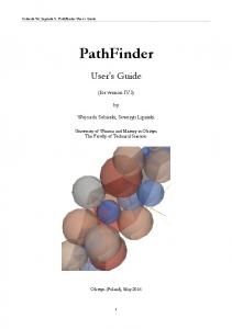
Figure 4: The pathfinder network (c) of the C. Elegans neural network, with the vertices size corresponding to the vertex degree in the MST. Highlighted in blue is the path between the nodes with the highest degree in the minimum spanning tree. It is easy to perceive the quantity of information that the MST removes when confronted with the PFNET.
Results are shown in Fig. 3: we report on the x-axis the size of the cluster (the number of workers) and on the y-axis a log scale of the running times in seconds. The missing data points in the chart refer to instances that could not be computed with the given number of workers for lack of resources (e.g. memory). The smallest graphs can be seen in the lowest part of the chart; in middle, we can find the graphs ranging from Email-EuAll up to Soc-Delicious. The largest graphs are shown in the upper part of the chart. GraphRay is able to tackle graphs with more than one million edges with as little as two machines (e.g. Soc-Delicious graph). As more machines are added, our algorithm could tackle larger and larger graphs up to 28 million edges. The running times are below 1,000 secs for graphs with less than 5M edges and below 1,400 secs for graphs with 20M or more edges. When increasing the size of the cluster to five machines, the average decrease in running times is about 55% compared to the 2-worker case. From five to ten workers, the average decrease is less noticeable, 45%, but still noteworthy. Increasing the cluster size to 15 leads to a 24% average reduction of the runtimes. Finally, with 20 workers, the average running times decrease by 11%. In some cases, like Soc-Delicious, we can show that the decrease in the running times is close to linear with the number of machines, going from 508 secs with 2 machines to 58 secs with 20. For smaller graphs, such as the first six of Table 1, visible at the bottom of the chart, the running times aren’t affected by the size of the cluster. Instead, the running times tend to increase as more machines are added. The reason of this behavior lies in the distributed environment, rather than in our implementation. When small graphs (few thousands of edges) are computed on a large cluster, the input is split into very small chunks and distributed over the workers. Larger clusters have higher costs in terms of synchronization traffic and I/O operations. In general, with a small
(a)
(b)
Figure 5: A comparison of the connections between a small group of vertices in our C. Elegans [44] case study as visualized by the MST (a) and our pruned graph (b). The second unveils an otherwise removed structure difficult to spot into the original graph. The thickness of an edge represents its relative weight.
portion of vertices on each machine, the overhead imposed by the infrastructure will balance the benefits of the distributed environment. It is possible to observe this behavior for the graphs ranging from CA-GrQc to Gnutella31. This behavior tends to fade as the graph size increases, but at the same time, we can see how the running times tend to stabilize after 15 machines, suggesting that as the balance point between costs and benefits for that range of graphs. We can conclude that distributed environments are not suited for small graphs, and, at the same time, to ensure maximum efficiency the number of machines composing the cluster must be chosen based on the size of the graph to compute. Overall, our implementation is scalable and able to tackle large graphs with reasonable running times. GraphRay also shows good efficiency, requiring a small number of machines even for large instances. 5
C ASE S TUDIES
To show how PFNETs impact on the visualization of real weighted networks, we select three different real weighted undirected networks: for each one of them we extract the PFNET (r = ∞, q = n −1) using GraphRay. We visualize both the layout of the whole graph and the one of its corresponding PFNET, computed by the ForceAtlas 2 algorithm [23] (unless differently stated), using the same visualization technique. We then discuss how resultant visualizations are changed. Each dataset has been stripped of its smaller connected components (if any), leaving only the largest one. All the graphs are freely available on the internet4 . 5.1
C. Elegans Neural Network
We applied our technique to the visualization of C. Elegans nematode neural network (Fig. 4). This organism has been extensively studied and is the first one whose neural connections were all mapped [46]. This dataset was collected by Watts and Strogatz [44] and counts 297 vertices and 2,148 edges. Its vertices represent the neurons of the worm, and the edges its neural links. The corresponding PFNET counts 947 edges (56% reduction from the original graph). We compared our result with the full graph and its MST. It is evident how the MST effectively shows a skeletal structure of the graph, with its high degree vertices coloured in blue, with a prevalence of star nodes (high degree nodes with many one-degree vertex neighbours). The visualization is less cluttered, but even though it provides an insight of the most important neurons of the brain, we find two major drawbacks: the first one is, given that we did not assume the edge weights to be distinct, there can be multiple 4 http://www-personal.umich.edu/˜mejn/netdata/
(a)
(b)
Figure 6: Rendering of Cond-Mat-2005 dataset [32] (a) and its corresponding PFNET (b) computed by LaGO [47]. The pruned network visualization provides much more insight about the underlying co-citation structure than its full graph counterpart. A few authors in key spots have been highlighted as reference points. The difference in the size of the label follows the change in the vertices degree.
spanning trees, with that one being only one of the possibile MSTs of that network. Second, the loss of potential useful information: even if we have a basic visualization of the brain connections, we cannot infer if there are other paths connecting those edges or see any other meaningful structure. To ease the comparison, we coloured the path connecting the four vertices with the highest degree in the MST in blue and highlighted it in all the figures. The PFNET yields a reduced-clutter visualization when compared to the layout of the full graph, while including much more information than the MST. Other than the path found in the MST, we can find several other paths connecting those vertices. The abundance of paths between that set of neurons suggests
(a)
(b)
Figure 7: Closeup of the LaGO rendering of the Havlin cluster in condensed matter collaboration network: full graph (a) versus PFNET (b).
the resilience by redundancy of that simple structure. This allows primitive organisms, such as the C. Elegans nematode, to survive even in the harshest conditions. Furthermore, our sparsified network also conveys information about other structures and connections otherwise hidden (see Fig. 5). 5.2
Condensed Matter Collaboration Network
The condensed matter collaboration network is a dataset consisting of 36,458 vertices and 171,375 edges [32]. The graph represents the coauthorships between researchers posting preprints on the “Condensed Matter E-Print archive5 ”. As reported by Newman [32], this graph has a small-world structure, meaning that it presents a combination of high clustering with short characteristic path length. A layout of this kind of graphs usually results in a “hairball”, a dense, ball-like drawing unable to convey any information whatsoever. To visualize the network, we choose the “LArge Graph Observer” (LaGO) software presented by Zinsmaier et al. [47]. This software allows an interactive visualization of the graph, following a details on-demand interaction. It combines edge cumulation with densitybased node aggregation. Our comparison is shown in Fig. 6a. The different shades of blue represent the vertex density, with denser areas coloured with a darker tone than the sparser ones. Edges are bundled together and the size of each bundle is color-coded with different shades of orange (lighter means fewer edges than the darker ones). The extracted the PFNET of the network, totals 91,513 edges (47% reduction) and its layout is shown in Fig. 6b. To ease the comparison, we selected a few vertices (authors) with the highest degree. The larger the label is, the higher degree of the vertex. With a simple inspection, we immediately find the presence of three major clusters, named after three researchers among the ones with the highest degree: Sarrao for the top one, Scheffler for 5 https://arxiv.org/archive/cond-mat
(a)
(b)
Figure 8: Comparison between the layout of the whole Astro-Ph dataset [32] (a) and the drawing of its PFNET. Both the drawings were computed by the algorithm described by Didimo and Montecchiani [16]. Thanks to our sparsification, the connections between the clusters are now much more easy to spot, and also the internal structure of each cluster is much more visible. The biggest 5 clusters are still visible and this proves how this technique does not change the overall structure of the graph.
the middle one and Havlin for the bottom one. The first remark we make is that in Fig. 6b the presence of Scheffler cluster appear to be more recognizable than in Fig. 6a. Secondly, more details of Sarrao cluster can be observed in the PFNET rendering than in its full counterpart. Particular attention should be given to the Havlin cluster, which can be seen in more detail in Fig. 7. Fig. 7b is a clearer picture and gives a precise idea of how the three authors are connected. 5.3 Astrophysics Collaboration Network This dataset represents a co-authorship network of researchers posting preprints on the Astrophysics E-Print archive6 . It is a weighted undirected network. It has 14,845 vertices and 119,652 edges [32]. We evaluate how the layout of the PFNET differs from the original when using a drawing algorithm able to find and highlight communities. We used a technique specifically designed to extract the clusters of small-world networks. First described by Didimo and Montecchiani [16], it combines a space-filling technique with a fast force directed layout algorithm. The algorithm arranges each cluster into a rectangular region with an area proportional to its number of vertices. A treemap is used to assign each space to the corresponding cluster, and its layout will be computed right afterwards; the area of the drawing will be limited to the space assigned to the specific cluster. The boundaries of the area of each cluster are stroked red in the final layout. The result is an effective visualization of the set of the clusters in the network. The drawing computed by the algorithm on the astrophysics collaboration network is shown in Fig. 8a. The picture reveals the presence of 5 large clusters, placed on the corners of a polygon, connected to each other by several edges; in between, the underlying structure remains unknown for the most part. The PFNET of this network has 62,325 edges (48% reduction) and its layout is depicted in Fig. 8b. The two layouts appear to be 6 http://arxiv.org/archive/astro-ph
similar, with the 5 clusters previously identified still visible. Given the less cluttered visualization is possibile to distinguish more details concerning the inter-cluster connections, previously hidden. 6
C ONCLUSIONS
AND
F UTURE W ORK
We have introduced the first distributed algorithm for network sparsification based on pathfinder network scaling. We have designed and implemented the algorithm on Giraph, showing that our approach is scalable and able to tackle large graphs efficiently using the resources of the distributed environment. We show how our technique can successfully sparsify networks with millions of nodes in minutes, extending the use of this technology on large graphs. We also apply our technique to different graphs and we showed how the visual clutter can be reduced, unveiling hidden or hard to spot structures. The software is open-source and freely available online7 . We plan to further improve the performance of G RAPH R AY and expand the current experimentation. In particular, it would be helpful to find out if this approach can also be used for speeding up other graph related tasks, such as the computation of a layout or the process of calculating metrics. We plan to investigate the use of GraphRay on large dynamic graphs. Furthermore, we would like to know if GraphRay could improve the user interaction with large graphs, given its ability to tackle large instances quickly. ACKNOWLEDGMENTS This research is sponsored in part by the U.S. Department of Energy via grants DE-SC0007443 and DE-SC0012610. We would like to thank the anonymous reviewers for their valuable comments and suggestions. This paper is dedicated to the loving memory of Maria Domenica Gentile (1925–2017). 7 http://graphray.graphdrawing.cloud
R EFERENCES [1] K. J. Ahn, S. Guha, and A. McGregor. Analyzing graph structure via linear measurements. In Proceedings of the twenty-third annual ACMSIAM symposium on Discrete Algorithms, pages 459–467. Society for Industrial and Applied Mathematics, 2012. [2] K. J. Ahn, S. Guha, and A. McGregor. Graph sketches: sparsification, spanners, and subgraphs. In Proceedings of the 31st ACM SIGMODSIGACT-SIGAI symposium on Principles of Database Systems, pages 5–14, 2012. [3] G. R. Andrews. Foundations of multithreaded, parallel, and distributed programming, volume 11. Addison-Wesley Reading, 2000. [4] C. Avery. Giraph: Large-scale graph processing infrastructure on hadoop. Proceedings of the Hadoop Summit. Santa Clara, 11, 2011. [5] D. Battista G, P. Eades, I. G. Tollis, and R. Tamassia. Graph drawing: algorithms for the visualization of graphs. 1999. [6] U. Brandes, M. Arlind Nocaj, and U. Ortmann. Untangling the hairballs of multi-centered, small-world online social media networks. Journal of Graph Algorithms and Applications, (2), 2015. [7] A. E. Brouwer and W. H. Haemers. Spectra of graphs. Springer Science & Business Media, 2011. [8] J. W. Buzydlowski. A comparison of self-organizing maps and pathfinder networks for the mapping of co-cited authors. PhD thesis, Drexel University, 2002. [9] C. Chen. Bridging the gap: The use of pathfinder networks in visual navigation. Journal of Visual Languages & Computing, 9(3):267–286, 1998. [10] C. Chen. Generalised similarity analysis and pathfinder network scaling. Interacting with computers, 10(2):107–128, 1998. [11] C. Chen. Information visualisation and virtual environments. Springer Science & Business Media, 2013. [12] C. Chen, J. Kuljis, and R. J. Paul. Visualizing latent domain knowledge. IEEE Transactions on Systems, Man, and Cybernetics, Part C (Applications and Reviews), 31(4):518–529, 2001. [13] C. Chen and S. Morris. Visualizing evolving networks: Minimum spanning trees versus pathfinder networks. In Information Visualization, 2003. INFOVIS 2003. IEEE Symposium on, pages 67–74. IEEE, 2003. [14] T. H. Cormen, C. E. Leiserson, R. L. Rivest, and C. Stein. Introduction to algorithms second edition. The MIT Press, 2001. [15] W. Didimo and G. Liotta. Mining graph data. Graph Visualization and Data Mining, pages 35–64. [16] W. Didimo and F. Montecchiani. Fast layout computation of hierarchically clustered networks: Algorithmic advances and experimental analysis. In Information Visualisation (IV), 2012 16th International Conference on, pages 18–23. IEEE, 2012. [17] S. Fortunato. Community detection in graphs. Physics reports, 486(3):75–174, 2010. [18] W. S. Fung, R. Hariharan, N. J. Harvey, and D. Panigrahi. A general framework for graph sparsification. In Proceedings of the forty-third annual ACM symposium on Theory of computing, pages 71–80, 2011. [19] R. G. Gallager, P. A. Humblet, and P. M. Spira. A distributed algorithm for minimum-weight spanning trees. ACM Transactions on Programming Languages and systems (TOPLAS), 5(1):66–77, 1983. [20] J. A. Garay, S. Kutten, and D. Peleg. A sublinear time distributed algorithm for minimum-weight spanning trees. SIAM Journal on Computing, 27(1):302–316, 1998. [21] V. P. Guerrero-Bote, F. Zapico-Alonso, M. E. Espinosa-Calvo, R. G. Cris´ostomo, and F. de Moya-Aneg´on. Binary pathfinder: An improvement to the pathfinder algorithm. Information Processing & Management, 42(6):1484–1490, 2006. [22] S. Hauguel, C. Zhai, and J. Han. Parallel pathfinder algorithms for mining structures from graphs. In Data Mining, 2009. ICDM’09. Ninth IEEE International Conference on, pages 812–817. IEEE, 2009. [23] M. Jacomy, S. Heymann, T. Venturini, and M. Bastian. Forceatlas2, a graph layout algorithm for handy network visualization, 2012, 2014. [24] M. J¨unger and P. Mutzel. Graph drawing software. Springer Science & Business Media, 2012. [25] D. Kravitz. Two comments on minimum spanning trees. The Bulletin of the ICA, 49:7–10, 2007. [26] U. K. Kudikyala and R. B. Vaughn. Software requirement under-
[27] [28]
[29]
[30]
[31]
[32] [33]
[34]
[35]
[36]
[37]
[38]
[39]
[40] [41]
[42]
[43] [44] [45]
[46]
[47]
standing using pathfinder networks: discovering and evaluating mental models. Journal of Systems and Software, 74(1):101–108, 2005. J. Leskovec and A. Krevl. SNAP Datasets: Stanford large network dataset collection. http://snap.stanford.edu/data, June 2014. G. Lindner, C. L. Staudt, M. Hamann, H. Meyerhenke, and D. Wagner. Structure-preserving sparsification of social networks. In Proceedings of the 2015 IEEE/ACM International Conference on Advances in Social Networks Analysis and Mining 2015, pages 448–454. ACM, 2015. G. Malewicz, M. H. Austern, A. J. Bik, J. C. Dehnert, I. Horn, N. Leiser, and G. Czajkowski. Pregel: a system for large-scale graph processing. In Proc. of the 2010 ACM SIGMOD International Conference on Management of data, pages 135–146, 2010. R. R. McCune, T. Weninger, and G. Madey. Thinking like a vertex: a survey of vertex-centric frameworks for large-scale distributed graph processing. ACM Computing Surveys, 48(2):25, 2015. J. Neˇsetˇril, E. Milkov´a, and H. Neˇsetˇrilov´a. Otakar bor˚uvka on minimum spanning tree problem translation of both the 1926 papers, comments, history. Discrete mathematics, 233(1-3):3–36, 2001. M. E. Newman. The structure of scientific collaboration networks. Proc. of the National Academy of Sciences, 98(2):404–409, 2001. B. Nick, C. Lee, P. Cunningham, and U. Brandes. Simmelian backbones: Amplifying hidden homophily in facebook networks. In Advances in Social Networks Analysis and Mining (ASONAM), 2013 IEEE/ACM International Conference on, pages 525–532. IEEE, 2013. G. Pandurangan, D. Peleg, and M. Scquizzato. Message lower bounds via efficient network synchronization. In International Colloquium on Structural Information and Communication Complexity, pages 75–91. Springer, 2016. K. Patil and P. Brazdil. Text summarization: Using centrality in the pathfinder network. Int. J. Comput. Sci. Inform. Syst [online], 2:18–32, 2007. M. Purohit, B. A. Prakash, C. Kang, Y. Zhang, and V. Subrahmanian. Fast influence-based coarsening for large networks. In Proc. of the 20th ACM SIGKDD international conference on Knowledge discovery and data mining, pages 1296–1305, 2014. A. Quirin, O. Cord´on, V. P. Guerrero-Bote, B. Vargas-Quesada, and F. Moya-Aneg´on. A quick mst-based algorithm to obtain pathfinder networks (∞, n- 1). Journal of the American Society for Information Science and Technology, 59(12):1912–1924, 2008. A. Quirin, O. Cord´on, J. Santamar´ıa, B. Vargas-Quesada, and F. MoyaAneg´on. A new variant of the pathfinder algorithm to generate large visual science maps in cubic time. Information processing & management, 44(4):1611–1623, 2008. R. A. Rossi and N. K. Ahmed. The network data repository with interactive graph analytics and visualization. In Proc. of the TwentyNinth AAAI Conference on Artificial Intelligence, 2015. R. W. Schvaneveldt. Pathfinder associative networks: Studies in knowledge organization. Ablex Publishing, 1990. R. W. Schvaneveldt, F. T. Durso, and D. W. Dearholt. Network structures in proximity data. Psychology of learning and motivation, 24:249– 284, 1989. S. M. Shope, J. A. DeJoode, N. J. Cooke, and H. Pedersen. Using pathfinder to generate communication networks in a cognitive task analysis. In Proceedings of the Human Factors and Ergonomics Society Annual Meeting, volume 48, pages 678–682. SAGE Publications, 2004. L. G. Valiant. A bridging model for parallel computation. Communications of the ACM, 33(8):103–111, 1990. D. J. Watts and S. H. Strogatz. Collective dynamics of smallworldnetworks. Nature, 393(6684):440–442, 1998. H. D. White. Pathfinder networks and author cocitation analysis: A remapping of paradigmatic information scientists. Journal of the American Society for Information Science and Technology, 54(5):423–434, 2003. J. G. White, E. Southgate, J. N. Thomson, and S. Brenner. The structure of the nervous system of the nematode caenorhabditis elegans. Philos Trans R Soc Lond B Biol Sci, 314(1165):1–340, 1986. M. Zinsmaier, U. Brandes, O. Deussen, and H. Strobelt. Interactive level-of-detail rendering of large graphs. IEEE Transactions on Visualization and Computer Graphics, 18(12):2486–2495, 2012.