set programming [8] graphs are used for deciding whether answer sets exist [6]. ...... Kathrin Konczak et al. 6. A. 3!#¦. Qt S 4u¨ A. 3. @Ч y. BВ4u¨ A. 3. @ ;. 7. A. 3!#
Graphs and colorings for answer set programming: Abridged Report Kathrin Konczak, Thomas Linke, and Torsten Schaub Institut f¨ur Informatik, Universit¨at Potsdam, Postfach 90 03 27, D–14439 Potsdam
Abstract. We investigate rule dependency graphs and their colorings for characterizing the computation of answer sets of logic programs. We start from a characterization of answer sets in terms of totally colored dependency graphs. To a turn, we develop a series of operational characterizations of answer sets in terms of operators on partial colorings. In analogy to the notion of a derivation in proof theory, our operational characterizations are expressed as (non-deterministically formed) sequences of colorings, turning an uncolored graph into a totally colored one. This results in an operational framework in which different combinations of operators result in different formal properties. Among others, we identify the basic strategy employed by the noMoRe system and justify its algorithmic approach. Also, we distinguish Fitting’s and well-founded semantics.
1 Introduction Graphs constitute a fundamental tool within computing science. Similarly, in answer set programming [8] graphs are used for deciding whether answer sets exist [6]. We take the application of graphs further and elaborate upon using graphs as the underlying computational model for computing answer sets. To this end, we build upon the theoretical foundations introduced in [9, 1]. Accordingly, we are interested in characterizing answer sets by means of their set of generating rules. For determining, whether a rule belongs to this set, we must verify that each positive body atom is derivable and that no negative body atom is derivable. In fact, an atom is derivable, if the set of generating rules includes a rule, having the atom as its head; or conversely, an atom is not derivable, if there is no rule among the generating rules that has the atom as its head. Consequently, the formation of the set of generating rules boils down to resolving positive and negative dependencies among rules. For capturing these dependencies, we take advantage of the concept of a rule dependency graph, wherein each node represents a rule of the underlying program and two types of edges stand for the aforementioned positive and negative rule dependencies, respectively. For expressing the applicability status of rules, that is, whether a rule belongs to a set of generating rules or not, we color the respective nodes in the graph. In this way, an answer set can be expressed by a total coloring of the rule dependency graph. Of course, in what follows, we are mainly interested in the inverse, that is, when does a graph coloring correspond to an answer set of the underlying program; and, in particular, how can we compute such a total coloring. To this end, we start by identifying graph structures that allow for characterizing answer sets in terms of totally colored dependency graphs. We then build
138
Kathrin Konczak et al.
upon these characterizations for developing an operational framework for answer set formation. The idea is to start from an uncolored rule dependency graph and to employ specific operators that turn a partially colored graph gradually into a totally colored one that represents an answer set. This approach is strongly inspired by the concept of a derivation, in particular, that of an SLD-derivation [15]. Accordingly, a program has a certain answer set iff there is a sequence of operations turning the uncolored graph into a totally colored one, expressing the answer set. All proofs can be found in the full version of this abridged report [12].
2 Rules, programs, graphs, and colorings A logic program is a finite set of rules such as ������� �� � � ����������������� � � �� �������� , where ������� � , and each �!�" �$#&%'#&�)( is an atom. For such a rule * , we let +-,/.10 " *�( � 2 � 043 " *�( the body, 5 � � � �6 � �7���4�� �8�9� � � �����4�� ��: , denote the head, � " , of * and � � �
�
� �=: and 2 � 0�3?> " *�(�; " *�(aO
;A@ :
Next, we lay the graph-theoretical foundations of our approach. A graph is a pair
"6bc�ed ( where b is a set of vertices and d T bgfDb a set of (directed) edges. A graph "6bc�ed ( is acyclic if d contains no cycles. For hiT b , we denote d O " h f hj( by d J k . Also, we abbreviate lm; "6b Onh �Hd Jokp( by lqJ k . A subgraph of "rb'�ed ( is a graph " h �es ( such that htT b and s T d Jok . In the sequel, we are interested in graphs reflecting dependencies among rules. Definition 1. Let B be a logic program. The rule dependency graph (RDG) u " B �Hd`�I�Hd�� ( of B is a labeled directed graph with
d � w ; v d � ;wv
" * � 4* xy(`J * " * � *4xy(`J *
� * x)LpB � ?+ ,H.I0 � * x)LpB � ?+ ,H.I0 ] We omit the subscript B from u 6 " c b e � d context. An % -subgraph ( of u
" *4(`Ln2 � 40 3 � " *4(`Ln2 � 043�>
]
;
" *4xz( {}| " *4xz( {
whenever the underlying program is clear from the is a subgraph of u with d T dZ! for %'L�5^� � ~ : . For illustration, consider the logic program B � ;j5�* � � � �� *� : , where
� � * Z *^ �`�< The RDG
N� � �a x *�
� * I x ��)� �a
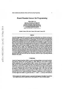
`� � *� (1) �* I ���H x � a � ]' of B � is depicted graphically in Figure 1a. The RDG u has among others
�
� �� �
� �� �
�� �
� ��� � � ��� � � � � �� �� �� � �
� � � ��
�
� � �
Graphs and� colorings:Abridged report � � � � 139 � �� � � � � � �
� ��� � � ��� ��� � ��� � � � � � � � � �� �� �� �� �� � � �
�� �� � � �� � � �� � � Fig. 1. (a) The RDG of logic program colored RDG �& �(' (partially) �! �%$ " � ; (b) The ". The totally colored RDG s ��� � and ��� �
��� � ��� � � � � �� �� �� �� � � �� � ��! �#" ; (c+d) �����
� -subgraph " 5^* � �� � * : � 5 " * ] � � * ( : ( and ~ -subgraph " 5�* � * : � 5 " * � * ( : ( . We call ) a coloring of u if ) is a mapping ) B+* 5-, �#. : . We denote the set ] of all partial colorings of a RDG u by /10-2 . For readability, we often omit the index ] u . Intuitively, the colors , and . indicate whether a rule is supposedly applied or blocked. We define )43R;j5�*$-J ) " *�(7;5, : and )46R;j5�*$J-) " *�(7; . : for obtaining all vertices colored by ) with , or . . If ) is total, " )73 � )46'( is a binary partition of B . That is, B 8 ; )93;:;)46 and )43 < O )=6 ; @ . Accordingly, we often identify a coloring ) with the pair " )93 � )46'( . A partial coloring ) induces a pair " )93 � )46'( of sets such that )43>:>)46gTgB and )43n> O )=6w; @ . For comparing partial colorings, ) and ) x , we define )@?A) x , if )43gB T ) 3 x and )46gA T ) 6 x . The “empty” coloring " @ � @1( is the ? -smallest coloring. Accordingly, we define )DCE) x as " )43;:E) 3 x � )=6F:E) 6 x ( . ] ] If ) is a coloring of u , we call the pair " u � )S( a colored RDG . For example, “coloring” the RDG of B � with ; " 5�* � � * : � 5^* : ( )
(2)
yields the colored graph in Figure 1b. For simplicity, when coloring, we replace the label of a node by the respective color. The central question addressed in this paper is how to compute the total colorings of RDG s that correspond to the answer sets of an underlying program. In fact, the colorings of interest can be distinguished in a straightforward way. Given a logic program B along E with its RDG u . Then, for every answer set of B , define an admissible coloring ) of u as )j;
" \Z] " E ( � BAG \�] " E ( (
By way of the respective generating rules, we associate with any program a set of admissible colorings whose members are in one-to-one correspondence with its answer E ; +?,H.I] 0 " ) 3 ( . We use sets. Clearly, any admissible coloring is total; also, we have X U " BD( for denoting the ] set of all admissible colorings of a RDG u .] For a partial " )S( as the set of all admissible colorings of u compatible coloring ) , we define X U with ) . Formally, given the RDG u of a logic program B and a partial coloring ) of u , define
] " ) (c;j5�) x L X U " D S B (`J-)8?H) x :
] " � ] " Clearly, ) � ?I)� implies X U ) (KJ X U )�^( . Observe that a partial coloring ) ] " is extendible to an admissible one ) x , that is, )B?L) x iff X U )S( is non-empty. For X U
140
Kathrin Konczak et al.
] " )S( is either empty or singleton. Regarding program B � and
a total coloring ) , X U coloring )� , we get
]' " � � �* � *^
: � ^5 * � �* � *� )� (';FX U " B � (c;G5 " 5^* 4 ] as shown in Figure 1c+d. Accordingly, define XZY " )S( of B compatible with partial coloring ) : E \ ] "E ] XZY " )S(7;G5 L XZY " BD(`J-) 3 T ( and ) 6 X U
E Note that +-,/.I0 " ) 3 (WT and coloring ) , we get
for any answer set
E
L XWY
: ( �� " ^5 * �� � ^* � *� : � ^5 *�
� *� � *� : ( : E as the set of all answer sets
\ ] "E (';F@ :
O
] " )S( . As regards program B �
] " )�^(7;AXZY " B � (c;G515 � 9�H : � 5 �6)�/ x :I:
XZY
We need the following concepts for describing a rule’s status of applicability. Definition 2. Let uR; " B �Hd � �ed � ( be the RDG of logic program B coloring of u . For *MLNB , we define:
�
and ) be a partial
1. * is supported in " u � )S( , if 2 � 0�3 " *�(8TA5�+-,/.10 " * x (KJ " * x � *�(8L d`�I� * x ; L )43 : ; " � " � ` d I � � " : 2. * is unsupported in u )S( , if 5^* x J * x *�($L +-,/.10 * x (S; T 4 ) 6 for some � �L 2 � 043 " *�( ; 3. * is blocked in " u � )S( , if * x L;) 3 for some " * x � *�(8L d � ; 4. * is unblocked in " u � )S( , if * x L;)46 for all " * x � *�(8L d�� .
�
�
�
��
�
In what follows, we use " u � )S( � " u � )S( � " u � )S( � and " u � )S( for denoting the sets of all supported, unsupported, blocked, and unblocked rules in " u � )S( . For illustration, ] � consider the sets obtained regarding the colored RDG " u )�^( in Figure 1b.
��"" u ]]' �� )�^(';j5�* � � *^ � *�
� * : u
)
(';F@
��"" u ]'] �� )��(c;G5�*^� :� u
)
(c;G5�*
* �* �* :
(3)
The next results are important for understanding the idea of our approach. Theorem 1. Let u be the RDG of logic program B E ] L XZY " )S( that Then, we have for every
� �
If ) 3. 4.
�
\ ] "E � �S ) (8T \ ] ( ;" E � )S(8T B G Z (. E : ] is admissible, we have for 5 ; XZY " S F ) ( that � \ ] E � )S(aO " u � )S(c; " (; � )S( : " u � )S(c;AB G \ ] " E ( .
"u �S ) (aO " u � )S( :
1. 2.
� �
"u "u
and ) be a partial coloring of u .
"u "u
� � �
Equation 3 and 4 are equivalent since ) is total. Reconsider the partially colored RDG " u ] � ) ( in Figure 1b. For every E L XZY ] " ) (c; 5I5 �6)�/ : � 5 � 9�H x :1: , we have
�
�
" u ] � ) (aO " u ]' � 7 ) ^( :
�
�
"u ] " u ]'
� ) (';G5^* � � * : T \ ] " E ( | \Z' ] "E
� )� (';G5^*� : T BBG � (
Graphs and colorings:Abridged report
141
3 Deciding answersetship from colored graphs The result in Theorem 1 started from an existing answer set induced from a given coloring. We now develop concepts that allow us to decide whether a (total) coloring represents an answer set by purely graph-theoretical means. To begin with, we define a graph structure accounting for the notion of recursive support. Definition 3. Let u be the RDG of logic program B and ) be a partial coloring of u . We define a support graph of " u � )S( as an acyclic � -subgraph "rb'�Hd ( of u such that �2 043 � " *�(KTP54+?,/.10 " * x (`J " * x � *�(8L d : for all * L b , ) 3 T b , and ) 6 O b ;A@ .
Every uncolored RDG (with ) ; " @ � @I( ) has a unique support graph possessing a largest set of vertices. We refer to such support graphs as maximal ones; all of them share the ] �^" � @ @1(e( , given same set of vertices. For example, the maximal support graph of " u in Figure 1a, excludes * , since it cannot be supported (recursively); otherwise, it con] tains, except for " * � *
( , all � -edges of u . The maximal support graph of the colored ] � ) ( , given in Figure 1b, is " 5^* � � * � *
� * : � 5 " * � � * ( ��" * � � * ( �^" * � *
( : ( . It RDG " u ]' � includes all positively colored and exclude all negatively colored nodes in " u )��( . : a “bad” coloring, like )G; " 5 � : � 5 : ( , may deny Given a program 5 � � the existence of a support graph of " u � )S( . As above, we distinguish maximal support graphs of colored graphs through their maximal set of vertices. For colored graphs, we have the following conditions guaranteeing the existence of (maximal) support graphs. Theorem 2. Let� u be the RDG of logic program B and ) be a partial coloring of u . ] " If X U )S( ;F@ , then there is a (maximal) support graph of " u � )S( . Clearly, the existence of a support graph implies that of a maximal one. Note furthermore that support graphs of totally colored graphs are necessarily maximal. Corollary 1. Let u be the RDG of logic program B and ) be an admissible coloring of u . Then, " ) 3 �ed ( is a support graph of " u � )S( for some d T " B f BD( . Taking the last result together with Property 3 or 4 in Theorem 1, we obtain a sufficient characterization of admissible colorings (along with their underlying answer sets). Theorem 3. Let u be the RDG of logic program B and let ) be a total coloring of u . Then, the following statements are equivalent.
�
1. ) is an admissible coloring of u ; " u � )S(aO " u � )S( and there is a support graph of 2. ) 3 ; " " u � )S( and there is a support graph of 3. )46 ; u � )S( :
�
�
�
"u �S ) (; " u � )S( .
For illustration, let us consider the two admissible colorings of RDG u ing to the two answer sets of program B � : )7��S;
" 5�* 4� � �* � *�
: � 5�* � *^ � *� : (
and
)7���;
]'
, correspond-
" 5^* �� � ^* � * : � 5^*�
� *� � *^ : ( (4)
The resulting colored RDG s are depicted in Figure 1c+d. Let us detail the case of )K�� :
�
�
] � "u ' )c��4(aO " u ] � ) �� ( :
�
�
] "u ' "u ]
� )c���(';j5�* � � ^* � *�
: ; " )c���( 8 3 | � ) �� (';j5�* � * � * : ; " ) �� ( 6
142
Kathrin Konczak et al.
]'
� )7��1( is given by " " )7��1(!3 � 5 " * �4� *� ( �^" *^ � *�
( : ( . The maximal support graph of " u In the full paper [12], we show how our graph-theoretical approach allows for capturing the original concepts like U � and B[C . Also, we introduce the concept of a blockage graph by means of ~ -subgraphs for capturing blockage relations.
4 Operational characterizations The goal of this section is to provide operational characterizations of answer sets. The idea is to start with the empty coloring " @ � @1( and to successively apply operators that turn a partial coloring ) into another one ) x such that )8?H) x , if possible. This is done until an admissible coloring, encompassing an answer set, is obtained. We concentrate first on operations deterministically extending partial colorings. Definition 4. Let u be the RDG of logic program B Then, define 0 / * / as 0
�
�
" )S('; ) C " " u � )S(aO " u � )S( �
�
and )
�
" u � )S( :
�� �
be a partial coloring of u .
" u � )S( (
0 " )S( . Note that 0 " )S( does A partial coloring ) is closed under 0 , if ) ; " " � ����� : � @I( ( would be " 5 � not always exist. To see this, observe that 70 5 ���4� : � 5 � ���4� : ( , which is no mapping and thus no partial coloring. Interestingly, 0 exists on colorings expressing answer sets.
� ��
�
Theorem 4. Let u be the RDG of logic program B � ] " If X U )S( ;F@ , then 0 " )S( exists.
�
��
and ) a partial coloring of u .
��
�� � �
] " )S(}; @ . To see this, consider B; 5 Note that 90 " )S( may exist although X U � K� � �a : . Clearly, X U ] " )S(c;F@ . However, 90 " " @ � @I( (c; " 5^* �4: � @I( exists. Now, we can define our principal propagation operator in the following way.
��
�
��
Definition 5. Let u be the RDG of logic program B and ) a partial coloring of u . Then, define 0 /H* / where 0 " )S( is the ? -smallest partial coloring containing ) and being closed under 70 .
�
Like 0 " )S( , 0 " )S( is not necessarily defined. This situation is made precise next.
�
Theorem 5. Let� u be the RDG of logic program B ] " )S( ;F@ , then 0 " )S( exists. If X U
�
and ) a partial coloring of u .
�
In fact, the non-existence of 0 is an important feature since an undefined application of 0 amounts to a backtracking situation at the implementation level. Note that ] "e" � "" � @ @1(e( ; @ (because of 0 @ @I( ( always exists, even though we may have X U XZY " BD(';A@ ). For illustration, consider program B � . We get:
�
0 "e" @ � " " � 0 �5 * : � �5 *^ e " " 0 5^* ��� *� : � �5 *^
@1(e(c; " �5 * � : � 5�*^ : ( : (e(c; " 5�* �� � ^* : � 5�*^ : (e(c; " 5�* ��� *^ : � �5 *^
: (
: ( and so 0
� " " @ � @I( (';
" 5^* � � �* : � �5 *� : (
Graphs and colorings:Abridged report
143
� �
Let us now elaborate upon the formal properties of 0 and 0 . First, we observe " 0 " )S( and ) ? that both are reflexive, that is, ) ? 0 )S( provided they exist. As shown in the full paper [12], � both operators are monotonic: For partial colorings ] " ) � ) x of u such that X U ) x ( ;�@ , we have: If ) ? ) x , then 90 " )S( ? 90 " ) x ( ; analogously for 0 . Consequently, we have ) ? 70 " )S( ? 90 " 90 " )S( ( . Moreover, ] " ] " " ] " " 40 and 0 are answer set preserving: X U )S(c; X U 40 )S(e(7;FX U 0 )S( ( . In fact, 90 can be used for deciding answersetship in the following way.
�
�
�
Corollary 2. Let u be the RDG of logic program B Then, ) is an admissible coloring of u iff 0 " )S(c;
�
)
and let ) be a total coloring of u . and " u � )S( has a support graph.
For relating 0 to the well-known Fitting operator [7], we need the following. Definition 6. Let u be the RDG of logic program B and let ) be a partial coloring of E � u . Define � ; 54+-,/.I0 " *�(NJ *RL )43 : and � ;�5 RJ for all *nLPB � if +?,H.I0 " *4(M; � then * L;)46 : .
E The pair "
� ] "E �� (
� �� � (
is a 3-valued interpretation of B . By letting the pair mapping be Fitting’s operator [7], we have the following result.
�
Theorem 6. Let u be the RDG of logic program B . "e" � @ (e( , then ���] " @ � @1('; " E � � � � ( . If ) ; 0 @ 1 A more detailed analysis of this relationship is given in the full paper [12]. The next operation draws upon the maximal support graph of colored RDG s. Definition 7. Let u be the RDG of logic program B and ) be a partial coloring of u . Furthermore, let "6bc�ed ( be a maximal support graph of " u � )S( for some d T " B f B[( . Then, define � 0 /H* / as
� 0
" )S(7; " ) 3 � BAG b (
This operator allows for coloring rules with . whenever it is clear from the given partial coloring that they will remain unsupported.1 Observe that B G b ; )96 : " BIG b ( . Like " 0 , � 0 )S( is an extension of ) . Unlike 0 , however, � 0 allows for coloring nodes unconnected with the already colored part of the graph. For B � , for instance, we obtain � 0 " " @ � @I( (`; " @ � 5�* : ( . While this information on * can also be supplied by 70 , it is � � : . In this case, not obtainable for “self-supporting 0-loops”, as in Bm;g5 � " " � " � � � � � : ( , which is not obtainable through 70 . we obtain � 0 @ @I( (c; @ 5 Operator � 0 is defined on colorings guaranteeing the existence of support graphs.
�
�
Corollary 3. Let u be the RDG of logic program B and ) be a partial coloring of u . If " u � )S( has a support graph, then � 0 " )S( exists.
We show in the full paper [12] that � 0 is reflexive, idempotent, monotonic, and� answer ] " )S( ;A@ and set preserving. That is, for partial colorings ) and ) x of u such that X U � ] " " " " " X U ) x ( ;�@ , we have ) ?�� 0 )S( , � 0 )S( ;�� 0 � 0 )S( ( , and if ) ? ) x , then ] ] � 0 " )S( ? � 0 " ) x ( . Moreover, we have X U " )S(M;�X U " � 0 " )S( ( . Note that unlike " � 0 , operator � 0 leaves the support graph of u )S( unaffected. Because � 0 implicitly enforces the existence of a support graph, our operators furnish yet another characterization of answer sets. 1
The relation to unfounded sets is detailed in the full paper [12].
144
Kathrin Konczak et al.
Corollary 4. Let u be the RDG of logic program B Then, ) is an admissible coloring of u iff )G;
and let ) be a total coloring of u . 0 " )S( and )G; � 0 " )S( .
��
��
Note that the last condition cannot guarantee that all supported unblocked rules belong to ) 3 . For instance, " @ � 5 � : ( has an empty support graph; hence " @ � 5 � : (; � 0 " " @ � 5 � : ( ( . That is, the trivially supported fact � remains in )76 . In our setting, such a miscoloring is detected by 0 . That is, 0 "e" @ � 5 � : ( ( is no partial coloring. Finally, we can express well-founded semantics [18] with our operators. For this, given a partial coloring ) , define " �S( 0 " )S( as the ? -smallest partial coloring containing ) and being closed under 0 and � 0 .
�
� ��
�
�
Theorem 7. Let u be the RDG of logic program B . E � If ) ; " �S( 0 " " @ � @1( ( , then " � � � ( is the well-founded model of B . A more detailed analysis of this relationship is given in the full paper [12]. We continue by providing a very general operational characterization that possesses a maximum degree of freedom. To this end, we observe that Corollary 4 can serve as a straightforward check for deciding whether a given total coloring constitutes an answer set. A corresponding guess can be provided through an operator capturing a non-deterministic (don’t know) choice. Definition 8. Let u be the RDG ��� of logic program B For � LD5-, �#. : , define 0 /H* / as 1. 2.
�
" )S(c; " ) 3 :D5�* : � ) 6 ( " " ) 3 � ) 6 : 5^* : ( 0 )S(c; 0
�
3 6
���
and )
be a partial coloring of u .
for some *MLQBAG " ) 3 : ) 6 ( ; for some *MLQBAG " ) 3 : ) 6 ( .
�
�
" " We use 0 � if � the distinction between 0 )S( and 0 )S( is of no importance. Strictly speaking, 0 is also parametrized with * ; we leave this implicit. Combining the previous guess and check operators yields our first operational characterization of admissible colorings (along with its underlying answer sets). 3
6
Theorem 8. Let u be the RDG of logic program B and let ) be a total coloring of u . ! Then, ) is an admissible coloring of u iff there exists a sequence " ) ( ����!���� where 1. 2. 3. 4. 5.
�
)
)
)
)
)
" � @1( ; ! ��; � @ � � � " � ; "0 ) � � ; � 0 ") � � ; 0 ) ; ) .
!
( for some � LD5-, �#. : and �M#&% �&� ;
(; (;
We refer to such sequences also as coloring sequences. Note that all sequences satisfying conditions 1-5 of Theorem 8 are successful insofar as their last element corresponds to an existing answer set. If a program has no answer set, then no such sequence exists. Although this guess and check approach is of no great implementational value, it supplies us with a skeleton for the coloring process that we refine in the sequel. In particular, it stresses the basic fact that we possess complete freedom in forming a coloring sequence as long as we can guarantee that the resulting coloring is a fixed point of 0 and � 0 . It is worth mentioning that this simple approach is inapplicable when fixing � to either , or . (see full paper [12]). We observe the following properties.
Graphs and colorings:Abridged report
145
!
Theorem 9. Given the prerequisites in Theorem 8, let " ) ( � ��! ��� be a sequence satisfying conditions 1-5 in Theorem 8. Then, we have the following properties for �M#�%7# � . 1. 2. 3. 4. 5.
!
) )
coloring; ! is a partial ! �9� ? ) ! ; ! �9� ] ] U ] ") !4 ( J� X U " ) (; U ! " ) ( ;P@ ; � ) ( has a (maximal) support graph.
X
X "u
All these properties represent invariants of � � the consecutive colorings. While the first three properties are provided by operator 0 in choosing among uncolored rules only, � the last two properties are actually enforced by the “check” on the final coloring ) expressed by conditions 3–5. In fact, sequences only enjoying conditions 1 and 2 in Theorem 8, fail to satisfy Property 4 and 5. In practical terms, this means that computations of successful sequences may be led numerous times on the “garden path”. As well-known, the number of choices can be significantly reduced by applying deterministic operators. Theorem 10. Let u be the RDG of logic program B and let ) be a total! coloring of u . Then, ) is an admissible coloring of u iff there exists a sequence " ) ( ����!���� where
��
�
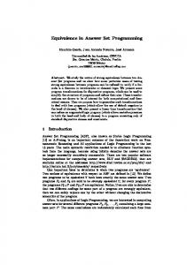
1. ) ! ��; � " �S( 0 " " @ � I ��@ � ( " ( ; ! " " ; �S( 0 0 ) (e( for some � LD5-, �#. : and �$#&% �&� ; 2. ) � 3. ) ; ) . The continuous applications of 0 and � 0 extend colorings after ! each choice. Furthermore, this proceeding guarantees that each partial coloring ) is closed under 0 and � 0 . It is clear in��� view of Theorem 8 that any number of iterations of � 0 and � 0 can be in Theorem 10. executed after 0 as long as " �S( 0 is the final operation leading to ) For illustration, consider the coloring sequence in Figure 2, obtained for answer set �6)�H x : of program B � . The decisive operation in this sequence is the application of �5 3 � 6 " 0 leading to ) *
(=; , . The same final result is obtained when choosing 0 such
�
� �
�
��
� �
�
�
� �� � � �� � � � � �� �� � � � � �
� �� �
�
� �
�
��
������� �
� �
�
� �� � � �� � � � � �� �� � � � �� � �� �
�
� �
�
��
���
� �
�
�
� �
�
� �� � ��� � � � � �� �� � � � �� � �� �
������� �
� �
�
��� � ��� � � � � �� �� ��� �� � �� �
Fig. 2. A coloring sequence.
that ) " * �('; . . So, several coloring sequences may lead to the same answer set. The usage of continuous propagations leads to further invariant properties.
!
Theorem 11. Given the prerequisites in Theorem 10, let " ) ( ����!���� be a sequence satisfying conditions 1-3 in Theorem 10. Then, we have properties 1–5 in Theorem 9 and
146
Kathrin Konczak et al.
�
! ���
6. ) 3 ! ��� J 7. ) 6 J
�
�
"u �) !a ( O " u � ) "u �) !( : "u �)
�
! !(; (.
Taking Property 6 and 7 together with 5 from Theorem 9, we see that propagation gradually enforces exactly the attributes on partial colorings, expressed in Theorem 3. Given that we obtain only two additional properties, one may wonder whether exhaustive propagation truly pays off. In fact, its value becomes apparent when looking at the properties of prefix sequences, not necessarily leading to a successful end. Theorem 12. Given the prerequisites in Theorem 10, let " ) ( ��� ��� be a sequence satisfying Condition 1 and 2 in Theorem 10. Then, we have properties 1–3, 5 in Theorem 9 and 6–7 in Theorem 11. Using exhaustive propagations, we observe that except for Property 4 all properties of successful sequences, are shared by (possibly unsuccessful) prefix sequences. In the full paper [12], we prove that propagation leads to shorter and fewer (prefix) sequences. What else may cut down the number of choices? Looking at the graph structures underlying an admissible coloring, we observe that support graphs possess a non-local, since recursive, structure, while blockage exhibits a rather local structure, based on arcwise constraints. Consequently, it seems advisable to prefer choices maintaining support structures over those maintaining blockage relations, since the former have more global repercussions than the latter. To this end, we develop in what follows a strategy that is based on a choice operation restricted to supported rules. Definition 9. Let u be the RDG � of logic program B For � LD5-, �#. : , define 0 /H* / as 1. 2.
" )S('; " 4 ) 3F: 5^* : � 4 ) 6'( 6 " " )43 � )46 :D5�* : ( 0 )S('; 0 �
�
3
�
for some * L for some * L
be a partial coloring of u .
�
and )
�
�
"u �S ) ( G " )93;: 4 ) 67( ; " u � )S( G " 9 ) 3;: 4 ) 67( .
� �
The number of rules colorable by� 0 is normally smaller than that by 0 . Depending on how the non-determinism of 0 is dealt with algorithmically, this may either lead to a reduced depth of the search tree or a reduced branching factor.� ! In a successful coloring sequence " ) ( � ��! ��� , all rules in ) 3 belong to an encom3 passing support graph. Furthermore, using 0 " )S( (and 0 ) the supportness of each set ! ) 3 is made invariant. Consequently, such a proceeding allows for establishing the existence of support graphs “on the fly” and offers a much simpler approach to the task(s) previously accomplished by � 0 . In fact, one may completely dispose of operator � 0 and color in a final step all uncolored rules with . . �
�
�
�
Definition 10. Let u be the RDG of logic program B and ) Then, define 0 / * / as 0 " )S(c; " )43 � BAG4)43'( . �
a partial coloring of u .
�
Roughly speaking, the idea is then to “actively” color only supported rules and rules blocked by supported rules; all remaining rules are then unsupported and “thrown” into ) 6 in a final step. Theorem 13. Let u be the RDG of logic program B and let ) be a total! coloring of u . Then, ) is an admissible coloring of u iff there exists a sequence " ) ( ����!���� where
Graphs and colorings:Abridged report
�
" � ! ��; � @ @1� ( ;" � ; " 0 )� � ; E0 " ) � � ; 0 ) ; ) .
)
1. 2. 3. 4. 5. )
�
)
�
) )
!
(� where � L[5 , � . : and �$#�% �&� > (; �
147
~;
(;
We note that there is a little price to pay for turning � 0 into E0 , expressed in Condition 4. Without it, one could use 0 to obtain a total coloring by coloring rules with . in an arbitrary way. We obtain the following properties for this type of sequences. �
�
!
Theorem 14. Given the prerequisites in Theorem 13, let " ) ( ����!���� be a sequence satisfying conditions 1-5 in Theorem 13. Then, we have properties 1–5 in Theorem 9 and
!
8. " ) 3 �Hd ( is a support graph of " u � )
!
( for some d T B
f B .
Unlike the coloring sequences only enjoying Condition 5 in Theorem 9, the sequences ! � formed by means of 0 guarantee that each ) 3 forms an independent support graph. 6 In fact, there is some overlap among operator 0 and E0 . To see this, consider B ;_5 � �/N� ���4� : . Initially, we must apply 03 to obtain " 5 � : � @1( from " @ � @1( . Then, however, we may either apply 6 or E0 for obtaining admissible coloring 0 " 5 : � 5 �� ����� : ( . Interestingly, this overlap can be eliminated by adding propagation operator 0 . This results in the basic strategy used in the noMoRe system [1]. �
��
��
�
� �
�
��
�
�
�
�
Theorem 15. Let u be the RDG of logic program B and let ) be a total! coloring of u . Then, ) is an admissible coloring of u iff there exists a sequence " ) ( ����!���� where 1. 2. 3. 4. 5.
�
)
)
! ��; � �
;
� ; )
)
)
0
; !
� � . : and �$#�% ��� � � ) ( ( where L[5 , " 0 ) � > (; 0 ") (; 0
�
� ;
� " �" @ " � @I� ( (" �
0
; ) .
~; �
�
Indeed, the strategy of noMoRe applies operator 0 as long as there are supported rules. Once no more uncolored supported rules exist, operator ;0 is called. Finally, 90 is applied but, in practice, only to those rules colored previously by 0 . At first sight, this approach may seem to correspond to a subclass of the coloring sequences described above, in the sense that noMoRe enforces a maximum number of transitions described in Condition 2 above. To see that this is not the case, we observe the following property. �
�
�
!
Theorem 16. Given the prerequisites in Theorem 15, let " ) � ( �� � ��!���� be� a� sequence satisfying conditions 1-5 in Theorem 15. Then, we have " 0 " ) > !( 6 G ) 6 > � ( T " u � )S( .
�
�
6
That is, no matter which (supported) rules are colored . by 0 , operator 0 only applies to unsupported� ones. It is thus no restriction to enforce the consecutive application of 0 and 0 until no more supported rules are available. In fact, it is the interplay of the two last operators that guarantees this property. For instance, looking at B ; 5 �/K� ���4� : , we see that we directly obtain the final total coloring because " 5 : � 5 � ���4� : ($; " 3 " " @ � @1( (e( , without any appeal to 0 . Rather it is 0 0 0 3 that detects that K� ����� is blocked. Generally speaking, 0 consecutively chooses
��
�
�
�
� � ��
�
�
�
�
�
�
148
Kathrin Konczak et al.
�
�
" u � )S('O " u � )S( . the generating rules of an answer set, finally gathered in )73 ; " � Clearly, every rule in u )S( is blocked by some rule in )73 . So whenever a rule * is 3 added by 0 to )43 , operator 0 adds all rules blocked by * to )96 . In this way, 0 and 3 " � " u � )S( and " u � )S( , so that all remaining 0 gradually color all rules in u )S()O uncolored rules, subsequently treated by F0 , must belong to " u � )S( . We obtain the following properties.
�
�
�
��
�
�
�
�
�
��
!
Theorem 17. Given the prerequisites in Theorem 15, let " ) ( ����!���� be a sequence satisfying conditions 1-5 in Theorem 15. Then, we have properties 1–5 in Theorem 9, 6–7 in Theorem 11, and 8 in Theorem 14. In the full paper [12], we discuss an alternative support-driven operational characterization using an incremantal version of �=0 instead of E0 . As well, we elaborate upon unicoloring strategies, using only one of the above choice operators instead of both. �
5 Discussion, related work, and conclusions Among the many graph-based approaches in the literature, we find some dealing with stratification [2], existence of answer sets [6, 3], or the actual characterization of answer sets or well-founded semantics [4, 3, 9, 11]. Our own approach has its roots in earlier work on default logic [13, 14, 17]. The usage of rule-oriented dependency graphs is common to [4, 3, 9]. In fact, the coloration of such graphs for characterizing answer sets was independently developed in [3] and [9]. While we borrow the term of an admissible coloring from the former, the work reported in Section 3 builds upon the latter and revises its definitions by appeal to the concept of a support graph. 2 Our major goal is however to provide an operational framework for answer set formation that allows us to bridge the gap between formal yet static characterizations of answer sets and algorithms for computing them. For instance, in the seminal paper [16] describing the smodels approach, answer sets are given in terms of so-called fullsets and their computation is directly expressed in terms of procedural algorithms. Our operational semantics aims at offering an intermediate stage that facilitates the formal elaboration of computational approaches. Our approach is strongly inspired by the concept of a derivation, in particular, that of an SLD-derivation [15]. This attributes our coloring sequences the flavor of a derivation in a family of calculi, whose respective set of inference rules correspond to the selection of operators. Although we leave out implementational issues, some remarks relating our approach, and thus the resulting noMoRe system [1], to the ones underlying dlv [5] and smodels [16] are in order. A principal difference manifests itself in how choices are performed. While the two latter’s choice is based on atoms occurring (negatively) in the underlying program, our choices are based on its rules. An advantage of our approach is that we can guarantee the support of rules on the fly. Unlike this, support checking is a recurring operation in the smodels system, similar to operator �40 . On 2
The definition of RDG s differs from that of “block graphs” in [9], whose practically motivated restrictions are superfluous from a theoretical perspective. Also, we abandon the latter term in order to give the same status to support and blockage relations.
Graphs and colorings:Abridged report
149
the other hand, this approach ensures that the smodels algorithm runs in linear space complexity, while a graph-based approach needs quadratic space in the worst case. This “investment” pays off once one is able to exploit the additional structural information offered by a graph. First steps in this direction are made in [10], where graph compressions are described that allow for conflating entire subgraphs into single nodes. Propagation is more or less done similarly in all three approaches. smodels relies on computing well-founded semantics, whereas dlv uses Fitting’s operator plus some backpropagation mechanisms. To sum up, we build upon the basic graph-theoretical characterizations in [9, 11] for developing an operational framework for non-deterministic answer set formation. The general idea is to start from an uncolored RDG and to employ specific operators that turn a partially colored graph gradually in a totally colored one, representing an answer set. To this end, we have developed a variety of deterministic and non-deterministic operators. Different coloring sequences (enjoying different formal properties) are obtained by selecting different combinations of operators. Among others, we have identified the particular strategy of the noMoRe system as well as operations yielding Fitting’s and wellfounded semantics. Taken together, the last results show that noMoRe’s principal propagation operation amounts to applying Fitting’s operator. Notably, the explicit detection of 0-loops is avoided by employing a support-driven choice operation. The noMoRe system is available at http://www.cs.uni-potsdam.de/ linke/nomore.
Acknowledgements The authors were partially supported by the German Science Foundation (DFG) under grant FOR 375/1 and SCHA 550/6, TP C and they were partially funded by the Information Society Technologies programme of the European Commission, Future and Emerging Technologies under the IST-2001-37004 WASP project.
References 1. C. Anger, K. Konczak, and T. Linke. noMoRe: Non-monotonic reasoning with logic programs. In S. Flesca et al., editors, Proceedings of the Eighth European Conference on Logics in Artificial Intelligence (JELIA’02), pages 521–524. Springer, 2002. 2. K. Apt, H. Blair, and A. Walker. Towards a theory of declarative knowledge. In J. Minker, editor, Foundations of Deductive Databases and Logic Programming, pages 89–148. Morgan Kaufmann, 1987. 3. G. Brignoli, S. Costantini, O. D’Antona, and A. Provetti. Characterizing and computing stable models of logic programs: the non-stratified case. In C. Baral and H. Mohanty, editors, Proceedings of the Conference on Information Technology, Bhubaneswar, India, pages 197– 201. AAAI Press, 1999. 4. Y. Dimopoulos and A. Torres. Graph theoretical structures in logic programs and default theories. Theoretical Computer Science, 170:209–244, 1996. 5. T. Eiter, N. Leone, C. Mateis, G. Pfeifer, and F. Scarcello. A deductive system for nonmonotonic reasoning. In J. Dix et al., editors, Proceedings of the Fourth International Conference on Logic Programming and Non-Monotonic Reasoning, pages 363–374. Springer, 1997.
150
Kathrin Konczak et al.
6. F. Fages. Consistency of clark’s completion and the existence of stable models. Journal of Methods of Logic in Computer Science, 1:51–60, 1994. 7. M. Fitting. Fixpoint semantics for logic programming a survey. Theoretical Computer Science, 278(1-2):25–51, 2002. 8. M. Gelfond and V. Lifschitz. Classical negation in logic programs and deductive databases. New Generation Computing, 9:365–385, 1991. 9. T. Linke. Graph theoretical characterization and computation of answer sets. In B. Nebel, editor, Proceedings of the International Joint Conference on Artificial Intelligence, pages 641–645. Morgan Kaufmann Publishers, 2001. 10. T. Linke. Using nested logic programs for answer set programming. 2003. Submitted. 11. T. Linke, C. Anger, and K. Konczak. More on noMoRe. In S. Flesca et al., editors, Proceedings of the Eighth European Conference on Logics in Artificial Intelligence (JELIA’02), pages 468–480, 2002. 12. T. Linke, K. Konczak, and T. Schaub. Graphs and colorings for answer set programming. Technical Report KRR-TR-03-01, University of Potsdam, June 2003. Available at http://www.cs.uni-potsdam.de/ torsten/Papers/KRR-TR-03-01.ps. 13. T. Linke and T. Schaub. An approach to query-answering in Reiter’s default logic and the underlying existence of extensions problem. In J. Dix et al., editors, Proceedings of the Sixth European Workshop on Logics in Artificial Intelligence, pages 233–247. Springer, 1998. 14. T. Linke and T. Schaub. Alternative foundations for Reiter’s default logic. Artificial Intelligence, 124(1):31–86, 2000. 15. J. Lloyd. Foundations of Logic Programming. Springer, 1987. 16. I. Niemel¨a and P. Simons. Efficient implementation of the well-founded and stable model semantics. In M. Maher, editor, Proceedings of the Joint International Conference and Symposium on Logic Programming, pages 289–303. The MIT Press, 1996. 17. C. Papadimitriou and M. Sideri. Default theories that always have extensions. Artificial Intelligence, 69:347–357, 1994. 18. A. van Gelder, K. Ross, and J. S. Schlipf. The well-founded semantics for general logic programs. Journal of the ACM, 38(3):620–650, 1991.