Tableau Calculi for Answer Set Programming

Tableau Calculi for Answer Set Programming Martin Gebser and Torsten Schaub Institut f¨ur Informatik, Universit¨at Potsdam, Postfach 90 03 27, D–14439 Potsdam

Abstract. We introduce a formal proof system based on tableau methods for analyzing computations made in Answer Set Programming (ASP). Our approach furnishes declarative and fine-grained instruments for characterizing operations as well as strategies of ASP-solvers. First, the granulation is detailed enough to capture the variety of propagation and choice operations of algorithms used for ASP; this also includes SAT-based approaches. Second, it is general enough to encompass the various strategies pursued by existing ASP-solvers. This provides us with a uniform framework for identifying and comparing fundamental properties of algorithms. Third, the approach allows us to investigate the proof complexity of algorithms for ASP, depending on choice operations. We show that exponentially different best-case computations can be obtained for different ASP-solvers. Finally, our approach is flexible enough to integrate new inference patterns, so to study their relation to existing ones. As a result, we obtain a novel approach to unfounded set handling based on loops, being applicable to non-SAT-based solvers. Furthermore, we identify backward propagation operations for unfounded sets.

1

Introduction

Answer Set Programming (ASP; [1]) is an appealing tool for knowledge representation and reasoning. Its attractiveness is supported by the availability of efficient off-the-shelf ASP-solvers that allow for computing answer sets of logic programs. However, in contrast to the related area of satisfiability checking (SAT), ASP lacks a formal framework for describing inferences conducted by ASP-solvers, such as the resolution proof theory in SAT-solving [2]. This deficiency led to a great heterogeneity in the description of algorithms for ASP, ranging over procedural [3, 4], fixpoint [5], and operational [6, 7] characterizations. On the one hand, this complicates identifying fundamental properties of algorithms, such as soundness and completeness. On the other hand, it almost disables formal comparisons among them. We address this deficiency by introducing a family of tableau calculi [8] for ASP. This allows us to view answer set computations as derivations in an inference system: A branch in a tableau corresponds to a successful or unsuccessful computation of an answer set; an entire tableau represents a traversal of the search space. Our approach furnishes declarative and fine-grained instruments for characterizing operations as well as strategies of ASP-solvers. In fact, we relate the approaches of assat, cmodels, dlv, nomore++, smodels, etc. [3, 4, 9, 7, 5] to appropriate tableau calculi, in the sense that computations of an aforementioned solver comply with tableau proofs in a corresponding calculus. This provides us with a uniform proof-theoretic framework for analyzing and comparing different algorithms, which is the first of its kind for ASP.

Based on proof-theoretic concepts, we are able to derive general results, which apply to whole classes of algorithms instead of only specific ASP-solvers. In particular, we investigate the proof complexity of different approaches, depending on choice operations. It turns out that, regarding time complexity, exponentially different bestcase computations can be obtained for different ASP-solvers. Furthermore, our prooftheoretic framework allows us to describe and study novel inference patterns, going beyond implemented systems. As a result, we obtain a loop-based approach to unfounded set handling, which is not restricted to SAT-based solvers. Also we identify backward propagation operations for unfounded sets. Our work is motivated by the desire to converge the various heterogeneous characterizations of current ASP-solvers, on the basis of a canonical specification of principles underlying the respective algorithms. The classic example for this is DPLL [10, 11], the most widely used algorithm for SAT, which is based on resolution proof theory [2]. By developing proof-theoretic foundations for ASP and abstracting from implementation details, we want to enhance the understanding of solving approaches as such. The proof-theoretic perspective also allows us to state results in a general way, rather than in a solver-specific one, and to study inferences by their admissibility, rather than from an implementation point of view. Our work is inspired by the one of J¨arvisalo, Junttila, and Niemel¨a, who use tableau methods in [12, 13] for investigating Boolean circuit satisfiability checking in the context of symbolic model checking. Although their target is different from ours, both approaches have many aspects in common. First, both use tableau methods for characterizing DPLL-type techniques. Second, using cut rules for characterizing DPLL-type split operations is the key idea for analyzing the proof complexity of different inference strategies. General investigations in propositional proof complexity, in particular, the one of satisfiability checking (SAT), can be found in [14]. From the perspective of tableau systems, DPLL is very similar to the propositional version of the KE tableau calculus; both are closely related to weak connection tableau with atomic cut (as pointed out in [15]). Tableau-based characterizations of logic programming are elaborated upon in [16]. Pearce, de Guzm´an, and Valverde provide in [17] a tableau calculus for automated theorem proving in equilibrium logic, based on its 5-valued semantics. Other tableau approaches to nonmonotonic logics are summarized in [18]. Bonatti describes in [19] a resolution method for skeptical answer set programming. Operator-based characterizations of propagation and choice operations in ASP can be found in [6, 7, 20].

2

Answer Set Programming

Given an alphabet P, a (normal) logic program is a finite set of rules of the form p0 ← p1 , . . . , pm , not pm+1 , . . . , not pn , where 0 ≤ m ≤ n and each pi ∈ P (0 ≤ i ≤ n) is an atom. A literal is an atom p or its negation not p. For a rule r, let head (r) = p0 be the head of r and body(r) = {p1 , . . . , pm , not pm+1 , . . . , not pn } be the body of r; and let body + (r) = {p1 , . . . , pm } and body − (r) = {pm+1 , . . . , pn }. The set of atoms occurring in a program Π is given by atom(Π). The set of bodies in Π is body(Π) = {body(r) | r ∈ Π}. For regrouping rule bodies with the same head p, let body(p) = {body(r) | r ∈ Π, head (r) = p}. A program Π is positive if body − (r) = ∅ for all

r ∈ Π. Cn(Π) denotes the smallest set of atoms closed under positive program Π. The reduct, Π X , of Π relative to a set X of atoms is defined by Π X = {head (r) ← body + (r) | r ∈ Π, body − (r) ∩ X = ∅}. A set X of atoms is an answer set of a logic program Π if Cn(Π X ) = X. As an example, consider Program Π1 = {a ←; c ← not b, not d; d ← a, not c} and its two answer sets {a, c} and {a, d}. An assignment A is a partial mapping of objects in a program Π into {T , F }, indicating whether a member of the domain of A, dom(A), is true or false, respectively. In order to capture the whole spectrum of ASP-solving techniques, we fix dom(A) to atom(Π) ∪ body(Π) in the sequel. We define AT = {v ∈ dom(A) | A(v) = T } and AF = {v ∈ dom(A) | A(v) = F }. We also denote an assignment A by a set of signed objects: {T v | v ∈ AT } ∪ {F v | v ∈ AF }. For instance with Π1 , the assignment mapping body ∅ of rule a ← to T and atom b to F is represented by {T ∅, F b}; all other atoms and bodies of Π1 remain undefined. Following up this notation, we call an assignment empty if it leaves all objects undefined. We define a set U of atoms as an unfounded set [21] of a program Π wrt a partial assignment A, if, for every rule r ∈ Π such that head (r) ∈ U , either (body + (r)∩AF )∪ (body − (r) ∩ AT ) 6= ∅ or body + (r) ∩ U 6= ∅. The greatest unfounded set of Π wrt A, denoted GUS (Π, A), is the union of all unfounded sets of Π wrt A. Loops are sets of atoms that circularly depend upon one another in a program’s positive atom dependency graph [3]. In analogy to external support [22] of loops, we define the external bodies of a loop L in Π as EB (L) = {body(r) | r ∈ Π, head (r) ∈ L, body + (r) ∩ L = ∅}. We denote the set of all loops in Π by loop(Π).

3

Tableau calculi

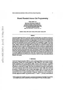
We describe calculi for the construction of answer sets from logic programs. Such constructions are associated with binary trees called tableaux [8]. The nodes of the trees are (mainly) signed propositions, that is, propositions preceded by either T or F , indicating an assumed truth value for the proposition. A tableau for a logic program Π and an initial assignment A is a binary tree such that the root node of the tree consists of the rules in Π and all members of A. The other nodes in the tree are entries of the form T v or F v, where v ∈ dom(A), generated by extending a tableau using the rules in Figure 1 in the following standard way [8]: Given a tableau rule and a branch in the tableau such that the prerequisites of the rule hold in the branch, the tableau can be extended by adding new entries to the end of the branch as specified by the rule. If the rule is the Cut rule in (m), then entries T v and F v are added as the left and the right child to the end of the branch. For the other rules, the consequent of the rule is added to the end of the branch. For convenience, the application of tableau rules makes use of two conjugation functions, t and f . For a literal l, define:   T l if l ∈ P T p if l = not p for a p ∈ P fl = tl = F p if l = not p for a p ∈ P F l if l ∈ P Some rule applications are subject to provisos. (§) stipulates that B1 , . . . , Bm constitute all bodies of rules with head p. (†) requires that p belongs to the greatest unfounded set induced by the rules whose bodies are not among B1 , . . . , Bm . (‡) makes sure that p

p ← l1 , . . . , ln tl1 , . . . , tln T {l1 , . . . , ln }

F {l1 , . . . , li , . . . , ln } tl1 , . . . , tli−1 , tli+1 , . . . , tln f li

(a) Forward True Body (FTB)

(b) Backward False Body (BFB)

p ← l1 , . . . , ln T {l1 , . . . , ln } Tp

p ← l1 , . . . , ln Fp F {l1 , . . . , ln }

(c) Forward True Atom (FTA)

(d) Backward False Atom (BFA)

p ← l1 , . . . , li , . . . , ln f li F {l1 , . . . , li , . . . , ln }

T {l1 , . . . , li , . . . , ln } tli

(e) Forward False Body (FFB)

(f) Backward True Body (BTB)

F B1 , . . . , F Bm (§) Fp

Tp F B1 , . . . , F Bi−1 , F Bi+1 , . . . , F Bm (§) T Bi

(g) Forward False Atom (FFA)

(h) Backward True Atom (BTA)

F B1 , . . . , F Bm (†) Fp

Tp F B1 , . . . , F Bi−1 , F Bi+1 , . . . , F Bm (†) T Bi

(i) Well-Founded Negation (WFN)

(j) Well-Founded Justification (WFJ)

F B1 , . . . , F Bm (‡) Fp

Tp F B1 , . . . , F Bi−1 , F Bi+1 , . . . , F Bm (‡) T Bi

(k) Forward Loop (FL)

(l) Backward Loop (BL)

Tv | Fv

(][X])

(m) Cut (Cut[X]) (§) (†) (‡) (][X])

: : : :

body(p) = {B1 , . . . , Bm } {B1 , . . . , Bm } ⊆ body(Π), p ∈ GUS ({r ∈ Π | body(r) 6∈ {B1 , . . . , Bm }}, ∅) p ∈ L, L ∈ loop(Π), EB (L) = {B1 , . . . , Bm } v∈X Fig. 1. Tableau rules for answer set programming.

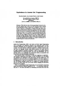
a← c ← not b, not d d ← a, not c T∅ Ta Fb Tc T {not b, not d} (h) Fd (f ) F {a, not c} (e)

Fc F {not b, not d} (d) Td (b) T {a, not c} (a)

(a) (c) (g) (Cut[atom(Π)])

Fig. 2. Tableau of Tsmodels for Π1 and the empty assignment.

belongs to a loop whose external bodies are B1 , . . . , Bm . Finally, (][X]) guides the application of the Cut rule by restricting cut objects to members of X.1 Different tableau calculi are obtained from different rule sets. When needed, this is made precise by enumerating the tableau rules. The following tableau calculi are of particular interest: Tcomp = {(a)-(h), Cut[atom(Π) ∪ body(Π)]} Tsmodels = {(a)-(i), Cut[atom(Π)]}

(1) (2)

TnoMoRe = {(a)-(i), Cut[body(Π)]}

(3)

Tnomore++ = {(a)-(i), Cut[atom(Π) ∪ body(Π)]}

(4)

An exemplary tableau of Tsmodels is given in Figure 2, where rule applications are indicated by either letters or rule names, like (a) or (Cut[atom(Π)]). Both branches comprise Π1 along with a total assignment for atom(Π1 ) ∪ body(Π1 ); the left one represents answer set {a, c}, the right one gives answer set {a, d}. A branch in a tableau is contradictory, if it contains both entries T v and F v for some v ∈ dom(A). A branch is complete, if it is contradictory, or if the branch contains either the entry T v or F v for each v ∈ dom(A) and is closed under all rules in a given calculus, except for the Cut rule in (m). For instance, both branches in Figure 2 are non-contradictory and complete. For each v ∈ dom(A), we say that entry T v (or F v) can be deduced by a set R of tableau rules in a branch, if the entry T v (or F v) can be generated from nodes in the branch by applying rules in R only. Note that every branch corresponds to a pair (Π, A) consisting of a program Π and an assignment A, and vice versa;2 we draw on this relationship for identifying branches in the sequel. Accordingly, we let DR (Π, A) denote ∗ (Π, A) the set of all entries deducible by rule set R in branch (Π, A). Moreover, DR represents the set of all entries in the smallest branch extending (Π, A) and being closed under R. When dealing with tableau calculi, like T , we slightly abuse notation and write DT (Π, A) (or DT∗ (Π, A)) instead of DT \{(m)} (Π, A) (or DT∗ \{(m)} (Π, A)), thus ignor∗ ing Cut. We mention that D{(a),(c),(e),(g)} (Π, A) corresponds to Fitting’s operator [23]. 1

2

The Cut rule ((m) in Figure 1) may, in principle, introduce more general entries; this would however necessitate additional decomposition rules, leading to extended tableau calculi. Given a branch (Π, A) in a tableau for Π and initial assignment A0 , we have A0 ⊆ A.

∗ Similarly, we detail in the subsequent sections that D{(a)-(h)} (Π, A) coincides with unit ∗ propagation on a program’s completion [24, 25], D{(a),(c),(e),(g),(i)} (Π, A) amounts to ∗ propagation via well-founded semantics [21], and D{(a)-(i)} (Π, A) captures smodels’ propagation [5], that is, well-founded semantics enhanced by backward propagation. Note that all deterministic rules in Figure 1 are answer set preserving; this also applies to the Cut rule when considering both resulting branches. A tableau is complete, if all its branches are complete. A complete tableau for a program and the empty assignment such that all branches are contradictory is called a refutation for the program; it means that the program has no answer set, as exemplarily shown next for smodels-type tableaux.

Theorem 1. Let Π be a logic program and let ∅ denote the empty assignment. Then, the following holds for tableau calculus Tsmodels : 1. Π has no answer set iff every complete tableau for Π and ∅ is a refutation. 2. If Π has an answer set X, then every complete tableau for Π and ∅ has a unique non-contradictory branch (Π, A) such that X = AT ∩ atom(Π). 3. If a tableau for Π and ∅ has a non-contradictory complete branch (Π, A), then AT ∩ atom(Π) is an answer set of Π. The same results are obtained for other tableau calculi, like TnoMoRe and Tnomore++ , all of which are sound and complete for ASP.

4

Characterizing existing ASP-solvers

In this section, we discuss the relation between the tableau rules in Figure 1 and wellknown ASP-solvers. As it turns out, our tableau rules are well-suited for describing the approaches of a wide variety of ASP-solvers. In particular, we cover all leading approaches to answer set computation for (normal) logic programs. We start with SATbased solvers assat and cmodels, then go on with atom-based solvers smodels and dlv, and finally turn to hybrid solvers, like nomore++, working on atoms as well as bodies. SAT-based solvers. The basic idea of SAT-based solvers is to use some SAT-solver as model generator and to afterwards check whether a generated model contains an unfounded loop. Lin and Zhao show in [3] that the answer sets of a logic program Π coincide with the models of the completion of Π and the set of all loop formulas of Π. The respective propositional logic translation is Comp(Π) ∪ LF (Π), where:3 W V Comp(Π) = {p ≡ ( k=1...m l∈Bk l) | p ∈ atom(Π), body(p) = {B1 , . . . , Bm }} V W V LF (Π) = {¬( k=1...m l∈Bk l) → p∈L ¬p | L ∈ loop(Π), EB (L) = {B1 , . . . , Bm }} This translation constitutes the backbone of SAT-based solvers assat [3] and cmodels [4]. However, loop formulas LF (Π) require exponential space in the worst case [26]. Thus, assat adds loop formulas from LF (Π) incrementally to Comp(Π), 3

Note that a negative default literal not p is translated as ¬p.

whenever some model of Comp(Π) not corresponding to an answer set has been generated by the underlying SAT-solver.4 The approach of cmodels avoids storing loop formulas by exploiting the SAT-solver’s inner backtracking and learning scheme. Despite the differences between assat and cmodels, we can uniformly characterize their model generation and verification steps. We first describe tableaux capturing the proceeding of the underlying SAT-solver and then go on with unfounded set checks. In analogy to Theorem 1, models of Comp(Π) correspond to tableaux of Tcomp . Theorem 2. Let Π be a logic program. Then, M is a model of Comp(Π) iff every complete tableau of Tcomp for Π and ∅ has a unique non-contradictory branch (Π, A) such that M = AT ∩ atom(Π). Intuitively, tableau rules (a)-(h) describe unit propagation on a program’s completion, represented in CNF as required by most SAT-solvers. Note that assat and cmodels introduce propositional variables for bodies in order to obtain a polynomially-sized set of clauses equivalent to a program’s completion [28]. Due to the fact that atoms and bodies are represented as propositional variables, allowing both of them as branching variables in Tcomp (via Cut[atom(Π) ∪ body(Π)]; cf. (1)) makes sense. Once a model of Comp(Π) has been generated by the underlying SAT-solver, assat and cmodels apply an unfounded set check for deciding whether the model is an answer set. If it fails, unfounded loops whose atoms are true (so-called terminating loops [3]) are determined. Their loop formulas are used to eliminate the generated model. Unfounded set checks, as performed by assat and cmodels, can be captured by tableau rules FFB and FL ((e) and (k) in Figure 1) as follows. Theorem 3. Let Π be a logic program, let M be a model of Comp(Π), and let A = {T p | p ∈ M } ∪ {F p | p ∈ atom(Π) \ M }. Then, M is an answer set of Π iff M ∩ (D{FL} (Π, D{FFB} (Π, A)))F = ∅. With SAT-based approaches, sophisticated unfounded set checks, able to detect unfounded loops, are applied only to non-contradictory complete branches in tableaux of Tcomp . Unfortunately, programs may yield exponentially many loops [26]. This can lead to exponentially many models of a program’s completion that turn out to be no answer sets [29]. In view of Theorem 3, it means that exponentially many branches may have to be completed by final unfounded set checks. Atom-based solvers. We now describe the relation between smodels [5] and dlv [9] on the one side and our tableau rules on the other side. We first concentrate on characterizing smodels and then sketch how our characterization applies to dlv. Given that only literals are explicitly represented in smodels’ assignments, whereas truth and falsity of bodies are determined implicitly, one might consider rewriting tableau rules to work on literals only, thereby, restricting the domain of assignments to atoms. For instance, tableau rule FFA ((g) in Figure 1) would then turn into: f l1 , . . . , f lm ({r ∈ Π | head (r) = p, body(r) ∩ {l1 , . . . , lm } = ∅} = ∅) Fp 4

Note that every answer set of Π is a model of Comp(Π), but not vice versa [27].

Observe that, in such a reformulation, one again refers to bodies by determining their values in the proviso associated with the inference rule. Reformulating tableau rules to work on literals only thus complicates provisos and does not substantially facilitate the description.5 In [29], additional variables for bodies, one for each rule of a program, are even explicitly introduced for comparing smodels with DPLL. Given that propagation, even within atom-based solvers, has to consider the truth status of rules’ bodies, the only saving in the computation of answer sets is limiting branching to atoms, which is expressed by Cut[atom(Π)] in Tsmodels (cf. (2)). Propagation in smodels is accomplished by two functions, called atleast and atmost [5].6 The former computes deterministic consequences by applying completionbased forward and backward propagation ((a)-(h) in Figure 1); the latter falsifies greatest unfounded sets (WFN ; (i) in Figure 1). The following result captures propagation via atleast in terms of Tcomp . Theorem 4. Let Π be a logic program and let A be an assignment such that AT ∪ AF ⊆ atom(Π). Let AS = atleast(Π, A) and AT = DT∗comp (Π, A). F T F If AT S ∩ AS 6= ∅, then AT ∩ AT 6= ∅; otherwise, we have AS ⊆ AT .

This result shows that anything derived by atleast can also be derived by Tcomp (withF out Cut). In fact, if atleast detects an inconsistency (AT S ∩ AS 6= ∅), then Tcomp can F T derive it as well (AT ∩AT 6= ∅). Otherwise, Tcomp can derive at least as much as atleast (AS ⊆ AT ). This subsumption does not only originate from the (different) domains of assignments, that is, only atoms for atleast but also bodies for Tcomp . Rather, it is the redundant representation of rules’ bodies within smodels that inhibits possible derivations obtained with Tcomp . To see this, consider rules a ← c, d and b ← c, d and an assignment A that contains F a but leaves atoms c and d undefined. For such an A, atleast can only determine that rule a ← c, d must not be applied, but it does not recognize that rule b ← c, d, sharing body {c, d}, is inapplicable as well. If b ← c, d is the only rule with head atom b in the underlying program, then Tcomp can, in contrast to atleast, derive F b via FFA ((g) in Figure 1). A one-to-one correspondence between atleast and Tcomp on derived atoms could be obtained by distinguishing different occurrences of the same body. However, for each derivation of atleast, there is a corresponding one in Tcomp . That is, every propagation done by atleast can be described with Tcomp . Function atmost returns the maximal set of potentially true atoms, that is, atom(Π) \ (GUS (Π, A) ∪ AF ) for a program Π and an assignment A. Atoms in the complement of atmost, that is, the greatest unfounded set GUS (Π, A) augmented with AF , must be false. This can be described by tableau rules FFB and WFN ((e) and (i) in Figure 1). Theorem 5. Let Π be a logic program and let A be an assignment such that AT ∪ AF ⊆ atom(Π). We have atom(Π) \ atmost(Π, A) = (D{WFN } (Π, D{FFB} (Π, A)))F ∪ AF . 5

6

Restricting the domain of assignments to atoms would also disable the analysis of different Cut variants in Section 5. Here, atleast and atmost are taken as defined on signed propositions instead of literals [5].

Note that smodels adds literals {F p | p ∈ atom(Π) \ atmost(Π, A)} to an assignment A. If this leads to an inconsistency, so does D{WFN } (Π, D{FFB} (Π, A)). We have seen that smodels’ propagation functions, atleast and atmost, can be described by tableau rules (a)-(i). By adding Cut[atom(Π)], we thus get tableau calculus Tsmodels (cf. (2)). Note that lookahead [5] can also be described by means of Cut[atom(Π)]: If smodels’ lookahead derives some literal tl, a respective branch can be extended by Cut applied to the atom involved in l. The subbranch containing f l becomes contradictory by closing it under Tsmodels . Also, if smodels’ propagation detects an inconsistency on tl, then both subbranches created by Cut, f l and tl, become contradictory by closing them; the subtableau under consideration becomes complete. After having discussed smodels, we briefly turn to dlv: In contrast to smodels’ atmost, greatest unfounded set detection is restricted to strongly connected components of programs’ atom dependency graphs [20]. Hence, tableau rule WFN has to be adjusted to work on such components.7 In the other aspects, propagation within dlv [6] is (on normal logic programs) similar to smodels’ atleast. Thus, tableau calculus Tsmodels also characterizes dlv very closely. Hybrid solvers. Finally, we discuss similarities and differences between atom-based ASP-solvers, smodels and dlv, and hybrid solvers, working on bodies in addition to atoms. Let us first mention that SAT-based solvers, assat and cmodels, are in a sense hybrid, since the CNF representation of a program’s completion contains variables for bodies. Thus, underlying SAT-solvers can branch on both atoms and bodies (via Cut[atom(Π) ∪ body(Π)] in Tcomp ). The only genuine ASP-solver (we know of) explicitly assigning truth values to bodies, in addition to atoms, is nomore++ [7].8 In [7], propagation rules applied by nomore++ are described in terms of operators: P for forward propagation, B for backward propagation, U for falsifying greatest unfounded sets, and L for lookahead. Similar to our tableau rules, these operators apply to both atoms and bodies. We can thus show direct correspondences between tableau rules (a), (c), (e), (g) and P, (b), (d), (f), (h) and B, and (i) and U. Similar to smodels’ lookahead, derivations of L can be described by means of Cut[atom(Π) ∪ body(Π)]. So by replacing Cut[atom(Π)] with Cut[atom(Π) ∪ body(Π)], we obtain tableau calculus Tnomore++ (cf. (4)) from Tsmodels . In the next section, we show that this subtle difference, also observed on SAT-based solvers, may have a great impact on proof complexity.

5

Proof complexity

We have seen that genuine ASP-solvers largely coincide on their propagation rules and differ primarily in the usage of Cut. In this section, we analyze the relative efficiency of tableau calculi with different Cut rules. Thereby, we take Tsmodels , TnoMoRe , and Tnomore++ into account, all using tableau rules (a)-(i) in Figure 1 but applying the Cut rule either to atom(Π), body(Π), or both of them (cf. (2–4)). These three calculi are of particular interest: On the one hand, they can be used to describe the strategies of ASP-solvers, as shown in the previous section; on the other hand, they also represent different paradigms, either atom-based, rule-based, or hybrid. So by considering these 7 8

However, iterated application of such a WFN variant leads to the same result as (i) in Figure 1. Complementing atom-based solvers, the noMoRe system [30] is rule-based (cf. TnoMoRe in (3)).

particular calculi, we obtain results that, on the one hand, are of practical relevance and that, on the other hand, apply to different approaches in general. For comparing different tableau calculi, we use well-known concepts from proof complexity [14, 12]. Accordingly, we measure the complexity of unsatisfiable logic programs, that is, programs without answer sets, in terms of minimal refutations. The size of a tableau is determined in the standard way as the number of nodes in it. A tableau calculus T is not polynomially simulated [14, 12] by another tableau calculus T 0 , if there is an infinite (witnessing) family {Π n } of unsatisfiable logic programs such that minimal refutations of T 0 for Π are asymptotically exponential in the size of minimal refutations of T for Π. A tableau calculus T is exponentially stronger than a tableau calculus T 0 , if T polynomially simulates T 0 , but not vice versa. Two tableau calculi are efficiency-incomparable, if neither one polynomially simulates the other. Note that proof complexity says nothing about how difficult it is to find a minimal refutation. Rather, it provides a lower bound on the run-time of proof-finding algorithms (in our context, ASP-solvers), independent from heuristic influences. In what follows, we provide families of unsatisfiable logic programs witnessing that neither Tsmodels polynomially simulates TnoMoRe nor vice versa. This means that, on certain instances, restricting the Cut rule to either only atoms or bodies leads to exponentially greater minimal run-times of either atom- or rule-based solvers in comparison to their counterparts, no matter which heuristic is applied. Lemma 1. There is an infinite family {Π n } of logic programs such that 1. the size of minimal refutations of TnoMoRe is linear in n and 2. the size of minimal refutations of Tsmodels is exponential in n. Lemma 2. There is an infinite family {Π n } of logic programs such that 1. the size of minimal refutations of Tsmodels is linear in n and 2. the size of minimal refutations of TnoMoRe is exponential in n. Family {Πan ∪ Πcn } witnesses Lemma 1 and {Πbn ∪ Πcn } witnesses Lemma 2:      a1 x ← c1 , . . . , cn , not x  x ← not x               c1 ← a1  b1 x ← a1 , b1   c1 ← b1  Πan = Πbn = Πcn = .. .. ..      . . .             an   cn ← bn x ← an , bn cn ← an bn

 ← not b1    ← not a1  .. .  ← not bn    ← not an

The next result follows immediately from Lemma 1 and 2. Theorem 6. Tsmodels and TnoMoRe are efficiency-incomparable. Given that any refutations of Tsmodels and TnoMoRe are as well refutations of Tnomore++ , we have that Tnomore++ polynomially simulates both Tsmodels and TnoMoRe . So the following is an immediate consequence of Theorem 6. Corollary 1. Tnomore++ is exponentially stronger than both Tsmodels and TnoMoRe .

The major implication of Corollary 1 is that, on certain logic programs, a priori restricting the Cut rule to either only atoms or bodies necessitates the traversal of an exponentially greater search space than with unrestricted Cut. Note that the phenomenon of exponentially worse proof complexity in comparison to Tnomore++ does not, depending on the program family, apply to one of Tsmodels or TnoMoRe alone. Rather, families {Πan }, {Πbn }, and {Πcn } can be combined such that both Tsmodels and TnoMoRe are exponentially worse than Tnomore++ . For certain logic programs, the unrestricted Cut rule is thus the only way to have at least the chance of finding a short refutation. Empirical evidence for the exponentially different behavior is given in [31]. Finally, note that our proof complexity results are robust. That is, they apply to any possible ASP-solver whose proceeding can be described by corresponding tableaux. For instance, any computation of smodels can be associated with a tableau of Tsmodels (cf. Section 4). A computation of smodels thus requires time proportional to the size of the corresponding tableau; in particular, the magnitude of a minimal tableau constitutes a lower bound on the run-time of smodels. This correlation is independent from whether an assignment contains only atoms or also bodies of a program: The size of any branch (not containing duplicate entries) is tightly bound by the size of a logic program. Therefore, exponential growth of minimal refutations is, for polynomially growing program families as the ones above, exclusively caused by the increase of necessary Cut applications, introducing an exponential number of branches.

6

Unfounded sets

We have analyzed propagation techniques and proof complexity of existing approaches to ASP-solving. We have seen that all approaches exploit propagation techniques amounting to inferences from program completion ((a)-(h) in Figure 1). In particular, SAT-based and genuine ASP-solvers differ only in the treatment of unfounded sets: While the former apply (loop-detecting) unfounded set checks to total assignments only, the latter incorporate (greatest) unfounded set falsification (WFN ; (i) in Figure 1) into their propagation. However, tableau rule WFN , as it is currently applied by genuine ASP-solvers, has several peculiarities: A. WFN is partly redundant, that is, it overlaps with completion-based tableau rule FFA ((g) in Figure 1), which falsifies atoms belonging to singleton unfounded sets. B. WFN deals with greatest unfounded sets, which can be (too) exhaustive. C. WFN is asymmetrically applied, that is, solvers apply no backward counterpart. In what follows, we thus propose and discuss alternative approaches to unfounded set handling, motivated by SAT-based solvers and results in [3]. Before we start, let us briefly introduce some vocabulary. Given two sets of tableau rules, R1 and R2 , we say ∗ that R1 is at least as effective as R2 , if, for any branch (Π, A), we have DR (Π, A) ⊆ 2 ∗ DR1 (Π, A). We say that R1 is more effective than R2 , if R1 is at least as effective as R2 , but not vice versa. If R1 is at least as effective as R2 and vice versa, then R1 and R2 are equally effective. Finally, R1 and R2 are orthogonal, if they are not equally effective and neither one is more effective than the other. A correspondence between two rule sets R1 ∪ R and R2 ∪ R means that the correspondence between R1 and R2 holds when D∗ takes auxiliary rules R into account as well.

We start with analyzing the relation between WFN and FFA, both falsifying unfounded atoms in forward direction. The role of FFB ((e) in Figure 1) is to falsify bodies that positively rely on falsified atoms. Intuitively, this allows for capturing iterated applications of WFN and FFA, respectively, in which FFB behaves neutrally. Taking up item A above, we have the following result. Proposition 1. Set of rules {WFN , FFB } is more effective than {FFA, FFB }. This tells us that FFA is actually redundant in the presence of WFN . However, all genuine ASP-solvers apply FFA as a sort of “local” negation (e.g. atleast of smodels and operator P of nomore++) and separately WFN as “global” negation (e.g. atmost of smodels and operator U of nomore++). Certainly, applying FFA is reasonable as applicability is easy to determine. (Thus, SAT-based solvers apply FFA, but not WFN .) But with FFA at hand, Proposition 1 also tells us that greatest unfounded sets are too unfocused to describe the sort of unfounded sets that truly require a dedicated treatment: The respective tableau rule, WFN , subsumes a simpler one, FFA. A characterization of WFN ’s effect, not built upon greatest unfounded sets, is obtained by putting results in [3] into the context of partial assignments. Theorem 7. Sets of rules {WFN , FFB } and {FFA, FL, FFB } are equally effective. Hence, one may safely substitute WFN by FFA and FL ((k) in Figure 1), without forfeiting atoms that must be false due to the lack of (non-circular) support. Thereby, FFA concentrates on single atoms and FL on unfounded loops. Since both tableau rules have different scopes, they do not overlap but complement each other. Proposition 2. Sets of rules {FFA, FFB } and {FL, FFB } are orthogonal. SAT-based approaches provide an explanation why concentrating on cyclic structures, namely loops, besides single atoms is sufficient: When falsity of unfounded atoms does not follow from a program’s completion or FFA, then there is a loop all of whose external bodies are false. Such a loop (called terminating loop in [3]) is a subset of the greatest unfounded set. So in view of item B above, loop-oriented approaches allow for focusing unfounded set computations on the intrinsically necessary parts. In fact, the more sophisticated unfounded set techniques applied by genuine ASP-solvers aim at circular structures induced by loops. That is, both smodels’ approach, based on “source pointers” [32], as well as dlv’s approach, based on strongly connected components of programs’ atom dependency graphs [20], can be seen as restrictions of WFN to structures induced by loops. However, neither of them takes loops as such into account. Having considered forward propagation for unfounded sets, we come to backward propagation, that is, BTA, WFJ , and BL ((h), (j), and (l) in Figure 1). Although no genuine ASP-solver currently integrates propagation techniques corresponding to WFJ or BL, as mentioned in item C above, both rules are answer set preserving. Proposition 3. Let Π be a logic program and let A be an assignment. Let B ∈ body(Π) such that T B ∈ D{WFJ } (Π, A) (or T B ∈ D{BL} (Π, A), respectively). Then, branch (Π, A∪D{WFN } (Π, A∪{F B})) (or (Π, A∪D{FL} (Π, A∪{F B})), respectively) is contradictory.

Both WFJ and BL ensure that falsifying some body does not lead to an inconsistency due to applying their forward counterparts. In fact, WFJ and BL are contrapositives of WFN and FL, respectively, in the same way as simpler rule BTA is for FFA. A particularity of supporting true atoms by backward propagation is that “global” rule WFJ is more effective than “local” ones, BTA and BL. Even adding tableau rule BTB ((f) in Figure 1), for enabling iterated application of backward rules setting bodies to true, does not compensate for the global character of WFJ . Proposition 4. Set of rules {WFJ , BTB } is more effective than {BTA, BL, BTB }. We conclude by discussing different approaches to unfounded set handling. Both SAT-based and genuine ASP-solvers apply tableau rules FFA and BTA, both focusing on single atoms. In addition, genuine ASP-solvers apply WFN to falsify more complex unfounded sets. However, WFN gives an overestimation of the parts of unfounded sets that need a dedicated treatment: SAT-based approaches show that concentrating on loops, via FL, is sufficient. However, the latter apply loop-detecting unfounded set checks only to total assignments or use loop formulas recorded in reaction to previously failed unfounded set checks. Such a recorded loop formula is then exploited by propagation within SAT-based solvers in both forward and backward direction, which amounts to applying FL and BL. A similar kind of backward propagation, by either WFJ or BL, is not exploited by genuine ASP-solvers, so unfounded set treatment is asymmetric. We however believe that bridging the gap between SAT-based and genuine ASP-solvers is possible by putting the concept of loops into the context of partial assignments. For instance, a loop-oriented unfounded set algorithm is described in [33].

7

Discussion

In contrast to the area of SAT, where the proof-theoretic foundations of SAT-solvers are well-understood [2, 14], the literature on ASP-solvers is generally too specific in terms of algorithms or solvers; existing characterizations are rather heterogeneous and often lack declarativeness. We address this deficiency by proposing a tableau proof system that provides a formal framework for analyzing computations of ASP-solvers. To our knowledge, this approach is the first uniform proof-theoretic account for computational techniques in ASP. Our tableau framework allows to abstract away implementation details and to identify valid inferences; hence, soundness and completeness results are easily obtained. This is accomplished by associating specific tableau calculi with the approaches of ASP-solvers, rather than with their solving algorithms. The explicit integration of bodies into assignments has several benefits. First, it allows us to capture completion-based and hybrid approaches in a closer fashion. Second, it allows us to reveal exponentially different proof complexities of ASP-solvers. Finally, even inferences in atom-based systems, like smodels and dlv, are twofold insofar as they must take program rules into account for propagation (cf. Section 4). This feature is simulated in our framework through the corresponding bodies. Although this simulation is sufficient for establishing formal results, it is worth noting that dealing with rules bears more redundancy than dealing with their bodies. Related to this, we have seen that rule-wise consideration of bodies, as for instance done in smodels’ atleast, can forfeit

derivations that are easily obtained based on non-duplicated bodies (cf. paragraph below Theorem 4). The tableau rules underlying atom-based and hybrid systems also reveal that the only major difference lies in the selection of program objects to branch upon. The branching rule, Cut, has a major influence on proof complexity. It is wellknown that an uncontrolled application of Cut is prone to inefficiency. The restriction of applying Cut to (sub)formulae occurring in the input showed to be an effective way to “tame” the cut [8]. We followed this by investigating Cut applications to atoms and bodies occurring in a program. The proof complexity results in Section 5 tell us that the minimal number of required Cut applications may vary exponentially when restricting Cut to either only atoms or bodies. For not a priori degrading an ASP-solving approach, the Cut rule must thus not be restricted to either only atoms or bodies. Note that these results hold for any ASP-solver (or algorithm) whose proceeding can be described by tableaux of a corresponding calculus (cf. end of Section 5). Regarding the relation between SAT-based and genuine ASP-solvers, we have seen in Section 6 that unfounded set handling constitutes the major difference. Though both approaches, as practiced by solvers, appear to be quite different, the aims and effects of underlying tableau rules are very similar. We expect that this observation will lead to convergence of SAT-based and genuine ASP-solvers, in the sense that the next generation of genuine ASP-solvers will directly incorporate the same powerful reasoning strategies that are already exploited in the area of SAT [2]. Acknowledgments. This work was supported by DFG (SCHA 550/6-4). We are grateful to Christian Anger, Philippe Besnard, Martin Brain, Yuliya Lierler, and the anonymous referees for many helpful suggestions.

References 1. Baral, C.: Knowledge Representation, Reasoning and Declarative Problem Solving. Cambridge University Press (2003) 2. Mitchell, D.: A SAT solver primer. Bulletin of the European Association for Theoretical Computer Science 85 (2005) 112–133 3. Lin, F., Zhao, Y.: ASSAT: computing answer sets of a logic program by SAT solvers. Artificial Intelligence 157(1-2) (2004) 115–137 4. Giunchiglia, E., Lierler, Y., Maratea, M.: A SAT-based polynomial space algorithm for answer set programming. In Delgrande, J., Schaub, T., eds.: Proceedings of the Tenth International Workshop on Non-Monotonic Reasoning. (2004) 189–196 5. Simons, P., Niemel¨a, I., Soininen, T.: Extending and implementing the stable model semantics. Artificial Intelligence 138(1-2) (2002) 181–234 6. Faber, W.: Enhancing Efficiency and Expressiveness in Answer Set Programming Systems. Dissertation, Technische Universit¨at Wien (2002) 7. Anger, C., Gebser, M., Linke, T., Neumann, A., Schaub, T.: The nomore++ approach to answer set solving. In Sutcliffe, G., Voronkov, A., eds.: Proceedings of the Twelfth International Conference on Logic for Programming, Artificial Intelligence, and Reasoning. Springer (2005) 95–109 8. D’Agostino, M., Gabbay, D., H¨ahnle, R., Posegga, J., eds.: Handbook of Tableau Methods. Kluwer Academic (1999) 9. Leone, N., Faber, W., Pfeifer, G., Eiter, T., Gottlob, G., Koch, C., Mateis, C., Perri, S., Scarcello, F.: The DLV system for knowledge representation and reasoning. ACM Transactions on Computational Logic (2006) To appear.

10. Davis, M., Putnam, H.: A computing procedure for quantification theory. Journal of the ACM 7 (1960) 201–215 11. Davis, M., Logemann, G., Loveland, D.: A machine program for theorem-proving. Communications of the ACM 5 (1962) 394–397 12. J¨arvisalo, M., Junttila, T., Niemel¨a, I.: Unrestricted vs restricted cut in a tableau method for Boolean circuits. Annals of Mathematics and Artificial Intelligence 44(4) (2005) 373–399 13. Junttila, T., Niemel¨a, I.: Towards an efficient tableau method for boolean circuit satisfiability checking. In Lloyd J., et al., eds.: Proceedings of the First International Conference on Computational Logic. Springer (2000) 553–567 14. Beame, P., Pitassi, T.: Propositional proof complexity: Past, present, and future. Bulletin of the European Association for Theoretical Computer Science 65 (1998) 66–89 15. H¨ahnle, R.: Tableaux and related methods. In Robinson, A., Voronkov, A., eds.: Handbook of Automated Reasoning. Elsevier and MIT Press (2001) 100–178 16. Fitting, M.: Tableaux for logic programming. J. Automated Reasoning 13(2) (1994) 175–188 17. Pearce, D., de Guzm´an, I., Valverde, A.: A tableau calculus for equilibrium entailment. In Dyckhoff, R., ed.: Proceedings of the Ninth International Conference on Automated Reasoning with Analytic Tableaux and Related Methods. Springer (2000) 352–367 18. Olivetti, N.: Tableaux for nonmonotonic logics. [8] 469–528 19. Bonatti, P.: Resolution for skeptical stable model semantics. J. Automated Reasoning 27(4) (2001) 391–421 20. Calimeri, F., Faber, W., Leone, N., Pfeifer, G.: Pruning operators for answer set programming systems. Technical Report INFSYS RR-1843-01-07, Technische Universit¨at Wien (2001) 21. van Gelder, A., Ross, K., Schlipf, J.: The well-founded semantics for general logic programs. Journal of the ACM 38(3) (1991) 620–650 22. Lee, J.: A model-theoretic counterpart of loop formulas. In Kaelbling, L., Saffiotti, A., eds.: Proceedings of the Nineteenth International Joint Conference on Artificial Intelligence, Professional Book Center (2005) 503–508 23. Fitting, M.: Fixpoint semantics for logic programming: A survey. Theoretical Computer Science 278(1-2) (2002) 25–51 24. Clark, K.: Negation as failure. In Gallaire, H., Minker, J., eds.: Logic and Data Bases. Plenum Press (1978) 293–322 25. Apt, K., Blair, H., Walker, A.: Towards a theory of declarative knowledge. In Minker, J., ed.: Found. of Deductive Databases and Logic Programming. Morgan Kaufmann (1987) 89–148 26. Lifschitz, V., Razborov, A.: Why are there so many loop formulas? ACM Transactions on Computational Logic (2006) To appear. 27. Fages, F.: Consistency of Clark’s completion and the existence of stable models. Journal of Methods of Logic in Computer Science 1 (1994) 51–60 28. Babovich, Y., Lifschitz, V.: Computing answer sets using program completion. Draft (2003) 29. Giunchiglia, E., Maratea, M.: On the relation between answer set and SAT procedures (or, between cmodels and smodels). In Gabbrielli, M., Gupta, G., eds.: Proceedings of the Twentyfirst International Conference on Logic Programming. Springer (2005) 37–51 30. Konczak, K., Linke, T., Schaub, T.: Graphs and colorings for answer set programming. Theory and Practice of Logic Programming 6(1-2) (2006) 61–106 31. Anger, C., Gebser, M., Schaub, T.: What’s a head without a body. In Brewka, G., ed.: Proceedings of the Seventeenth European Conference on Artificial Intelligence, IOS Press (2006) To appear. 32. Simons, P.: Extending and Implementing the Stable Model Semantics. Dissertation, Helsinki University of Technology (2000) 33. Anger, C., Gebser, M., Schaub, T.: Approaching the core of unfounded sets. In Dix, J., Hunter, A., eds.: Proceedings of the Eleventh International Workshop on Non-Monotonic Reasoning. (2006) To appear.