Greedy Methods in Plume Detection, Localization

17 Greedy Methods in Plume Detection, Localization and Tracking Huimin Chen

University of New Orleans, Department of Electrical Engineering 2000 Lakeshore Drive, New Orleans, LA 70148, USA

Open Access Database www.intechweb.org

1. Introduction Greedy method, as an efficient computing tool, can be applied to various combinatorial or nonlinear optimization problems where finding the global optimum is difficult, if not computationally infeasible. A greedy algorithm has the nature of making the locally optimal choice at each stage and then solving the subproblems that arise later. It iteratively makes one greedy choice after another, reducing each given problem into a smaller one. In other words, a greedy algorithm never reconsiders its choices. Clearly, greedy method often fails to find the globally optimal solution. However, a greedy algorithm can be proven to yield the global optimum for a given class of problems such as Kruskal's algorithm and Prim's algorithm for finding minimum spanning tree, Dijkstra's algorithm for finding single-source shortest path, and the algorithm for finding optimum Huffman tree [5]. Even for some optimization problems proven to be NP hard, a greedy algorithm may generate near optimal solution with high probability if one exploits the problem structure properly. In this chapter, we focus on the optimization problems arising from plume detection, localization and tracking and provide convincing argument on the usefulness of greedy algorithms. Detection, identification, localization, tracking and prediction of chemical, biological or nuclear propagation is crucial to battlefield surveillance and homeland security. In addition, post-accident management for public protection relies critically on detecting and tracing dangerous gas leakages promptly. The determination of source origins and release rates is useful for the forecast of gas concentration in the atmosphere and for the management staff to prioritize off-site evacuation plans. A lot of research has been focused on detecting and localizing single or multiple plume sources with autonomous vehicles [11] or sensor networks such as [22] for a vapor-emitting source, [2] for a nuclear source, and [14, 15] for a chemical source. In [12] the plume detection and localization problem is formulated as abrupt change detection using sparse sensor measurements. The development of a large scale testbed has been reported in [8] for plume detection, identification and tracking. In [3] dense sensor coverage has been used for radioactive source detection while [26] showed that using three error-free intensity sensors, one can identify the plume origin to any desired accuracy with high probability. Although this approach offers an effective solution with linear complexity of the hypothesis space, a major limitation is that the continuous time dynamic model of plume propagation has to be in the product form. Source: Advances in Greedy Algorithms, Book edited by: Witold Bednorz, ISBN 978-953-7619-27-5, pp. 586, November 2008, I-Tech, Vienna, Austria

306

Advances in Greedy Algorithms

When the sensing devices can not provide accurate plume concentration readings, plume tracking relies heavily on the sensor coverage instead of the physics-based propagation model. In this case, hidden Markov model (HMM) offers a flexible tool to model the uncertainty of plume propagation motion in the air. It has been applied to plume mapping in [11] and chemical detection in [23]. The main issue of HMM resides in the time varying state transition probabilities which are not readily available from the physics based plume propagation equation. A viable approach is to use the generalized HMM with fuzzy measure and fuzzy integral [20]. The resulting plume localization problem becomes finding the most likely source sequence based on a fuzzy HMM. Existing algorithms of Viterbi type [20, 21] can be very inefficient when the size of the hidden state is large. Recently, [19] showed that the average complexity of finding the maximum likelihood sequence can be much lower than that using Viterbi algorithm for an HMM in the high SNR regime. Motivated by the theoretical result in [19], we propose a decoding algorithm of greedy type to obtain a candidate source path and search only for state sequences within a constrained Hamming distance from the candidate plume path. Our method is applicable to a general class of fuzzy measures and fuzzy integrals being used in fuzzy HMM. We compare the localization error using our algorithm with that using fuzzy Viterbi algorithm in a plume localization scenario with randomly deployed sensors. Simulation results indicate that the proposed greedy algorithm is much faster than fuzzy Viterbi algorithm for plume tracing over a long observation sequence when the localization error probability is small. When the sensing devices provide fairly accurate concentration readings of the sources, one would expect that plume localization and release sequence estimation can be solved jointly. However, despite the abundant literature in plume detection [3, 23, 24] and localization [11, 30, 31], limited efforts have been made toward solving the joint problem of source localization and parameter estimation. The main reason is that even finding linear parameters related to the source release rate is an ill-posed problem and one has to impose certain regularization technique to avoid potential overfit. To solve the plume identification and parameter estimation jointly, we adopt the least squares technique based on the solution to the advection-diffusion equation [16, 17] and impose lp-regularization for 0 ≤ p ≤ 1 [4, 7] to characterize the sparsity of the unknown source release rate signal. We also discuss its advantage over the popularly used l2-regularization. The accuracy of source parameter estimation is examined for the cases where both the number of sources and the corresponding locations are unknown. Since the resulting optimization problem is nonlinear and involves both discrete and continuous variables, we apply a greedy approach to identify and localize one source at a time. It is very efficient and can be interpreted as greedy basis pursuit [13]. The rest of the chapter is organized as follows. Section 2 formulates the plume localization problem using multiple binary detection sensors as maximum likelihood decoding over fuzzy HMM. Greedy algorithm is applied to maximum likelihood sequence estimation where the complexity comes from the fine resolution of the quantized surveillance area. Section 3 introduces the joint plume localization and source parameter estimation problem. Greedy algorithm is applied to source identification where the computational complexity mainly comes from the aggregation of unknown number of sources. Section 4 presents a concluding summary and discusses when one can expect good performance using greedy method.

Greedy Methods in Plume Detection, Localization and Tracking

307

2. Sequence estimation using fuzzy hidden Markov model This section focuses on the maximum likelihood sequence estimation where the problem lends itself with a combinatorial structure similar to a decoding problem. We start with continuous time plume propagation model in Section 2.1 and then discuss the discrete time Markov approximation of the plume source as well as the sensor measurement model in Section 2.2. Section 2.3 presents the sequence estimation problem over a fuzzy hidden Markov model (HMM) using Viterbi and greedy heuristic algorithm. Section 2.4 provides simulation study on tracing a single plume source with unknown source location and initial releasing time. 2.1 Gaussian puff plume propagation model It is challenging to accurately model the spatial and temporal distribution of a contaminant released into an environment due to the inherent randomness of the wind velocities in turbulent flow. Here we adopt a continuous time plume propagation model of instantaneous release type given in [28]. A plume consisting of particles or gases has the concentration c satisfying the following continuity equation

where is the j-th component of the wind velocity; D is the molecular diffusion coefficient; R is the rate of particle generation depending on the temperature T; S is the rate of aggregation of particles at location x and time t. In a perfectly known wind field where one knows the wind velocities at all locations, there will not be any turbulent diffusion. However, due to the randomness of the wind velocities, one can only expect that the mean concentration to satisfy the atmospheric diffusion equation

where is the j-th component of mean wind velocity and Kjj is the eddy diffusivity assuming molecular diffusion is negligible relative to turbulent diffusion. Assuming S(x, t) = 0 (instantaneous release) without any boundary condition, one can obtain the closed form solution to the above partial differential equation, which in the two dimensional case is

where x and y are the axis of the Cartesian coordinate system centered at the plume origin. In practice, one may not have the knowledge of the mean wind velocity at any location and it can also be time varying. In order to accommodate the uncertainty due to the aggregation of the plume release and the wind turbulence, in the sequel, we consider a dynamic model with both time and spatial transition following a Markov chain. 2.2 Approximate plume propagation dynamics and measurement model We assume that the search region is partitioned into N cells indicating the possible origins of the plume source. The centroid of cell i is denoted by (qxi, qyi) for i = 1, …,N. Sensors are

308

Advances in Greedy Algorithms

homogeneous and randomly deployed in the search region. Time is discretized by the sensing interval Δt where chemical intensity is measured in the neighborhood of each sensor's location. If the intensity is above a predetermined threshold, then a sensor will declare its detection of chemical plume. Thus at any time instant k, a binary sequence yk is obtained from M sensors located at (rxi, ryi) indicating a possible chemical detection for i = 1, …,M. We assume that the flow velocity (vxi(k), vyi(k)) is also recorded by sensor i at time k (∀i, k). Denote by x(j)k the hidden state of cell j at time k taking binary values indicating whether it contains detectable chemicals. Denote by xk = [x(1)k x(2)k … x(N)k]’ the plume map at time k. Denote by y1:K = [y1 … yK] the detection sequence up to time K and, accordingly, x1:K = [x1 … xK] the possible plume sequence up to time K. The plume mapping problem can be written as finding the most likely plume sequence (1) where a statistical model between the state and observation sequence is assumed and the maximum likelihood (ML) criterion is used. From the ML estimate of the state sequence, one can identify the origin of the plume and its initial releasing time. Note that using the above formulation, one can also estimate the origins of multiple plumes at unknown and possibly different releasing times. The major difficulty lies in the availability of state and measurement model at any given time. 2.3 Fuzzy hidden Markov model and maximum likelihood decoding 2.3.1 Hidden Markov plume model Two methods are popularly used in modeling plume propagation: numerical solution to the advection-dispersion equation and random simulation [9]. In this section, we use random simulation to generate realistic plume propagation sequence when evaluating the state sequence estimation algorithm. In a hidden Markov plume model, the state sequence {xk} is assumed to be a Markov chain. At any time k, a cell i has a probability pb originating a new plume release if it contains no plume at k - 1. A cell i has a probability pc releasing the same amount of plume at time k if it contains a plume source at k -1. A cell j has detectable plume at time k coming from the source in cell i at time k - 1 with probability pd(i) depending on the source intensity Q and minimal detectable intensity C. Without the presence of wind, we have pd(i) = 0 for Gaussian plume if (2) where D is the diffusion coefficient. With known flow velocity at cell i, the detectable region can be modified accordingly. Thus we denote by A(k) the state transition probability matrix of size 2N×2N with element amn(k) indicating p(xk = n⏐xk-1 = m) where m and n represent two binary sequences of length N. For each sensor, the probability of false alarm is assumed to be very low when there is no detectable plume in its neighborhood. The detection probability depends on the distance d between the sensor location and the centroid of the nearest cell which contains detectable plume. The following crude model is assumed. (3)

Greedy Methods in Plume Detection, Localization and Tracking

309

where  is chosen such that the detection probability at the edge of the cell is 1-C/Q. Thus we have specified the observation model B of size 2N×2M for M sensors with element bnl indicating the probability p(yk = l⏐xk = n). The hidden Markov plume model is represented where π is the initial probability of the state. by the parameter vector Note that the hidden Markov plume model is nonstationary since the state transition matrix is time varying. The model parameter Λ is difficult to learn from experiments since it requires large training sets with various wind conditions. 2.3.2 Fuzzy hidden Markov model Fuzzy hidden Markov model (FHMM) is a natural extension of the classical hidden Markov model with fuzzy measure and fuzzy integral. The theoretical framework was first proposed in [20] and applied to handwritten word recognition in [21]. Here we briefly highlight the key components in FHMM and its advantage over a nonstationary hidden Markov plume model. FHMM replaces the probability measure used in the classical HMM with the fuzzy measure. A fuzzy measure μ on the state space X is a mapping from subset of X onto the unit interval μ: 2X → [0, 1] such that μ (φ) = 0, μ (X) = 1, and if E ⊂ F, then μ (E) ≤ μ (F). To combine the evidences from different sensor measurements, the concept of fuzzy integral is introduced to replace the classical probabilistic inference. For a discrete set X = {x1, …, xn}, the Choquet integral of a function h with respect to a fuzzy measure μ is computed as follows. (4) where h(x0) = 0, h(x1) ≤ h(x2) ≤ … ≤ h(xn) and (5) A conditional fuzzy measure on Y given X is a fuzzy measure (·⏐x) on Y for any given x ∈ X. For E ⊂ Y , the -induced fuzzy measure is computed by (6) With the above tools, a fuzzy hidden Markov model can be parameterized by where is the initial fuzzy density of the state; is the state transition matrix parameterized by fuzzy densities; is measurement matrix parameterized by fuzzy densities. Note that the fuzzy state transition matrix is no longer time varying. This simplifies the learning of model parameters significantly. On the other hand, FHMM preserves the non-stationary nature of plume propagation and the nonstationary behavior is achieved naturally by the nonlinear aggregation of sensor measurements using fuzzy integral [20]. 2.3.3 Viterbi algorithm for most likely sequence estimation For an HMM with parameter Λ, finding the most likely state sequence given the is often called maximum likelihood (ML) decoding. Viterbi algorithm observation guarantees obtaining the ML sequence with the following procedure [25].

310

Advances in Greedy Algorithms

For a fuzzy hidden Markov model, the most likely state sequence given the observation sequence can also be defined with properly chosen fuzzy measure and fuzzy integral. The resulting optimization problem can be written as (7) where is the extension of likelihood function in (13) with the conditional fuzzy measure. Note that the fuzzy likelihood function can be decomposed as follows. (8) Thus the decoding algorithm of Viterbi type can also be applied to FHMM. Specifically, the fuzzy Viterbi decoding procedure is as follows. (9) (10) (11) where (12) if Choquet integral is used with respect to a fuzzy measure μ [20]. It is a time varying and nonlinear function of the fuzzy state transition parameter , which characterizes the nonstationary nature of plume propagation using only time invariant parameter set . The resulting state sequence estimate is still given by

Note that the most likely sequence estimation algorithm of Viterbi type guarantees finding the optimal solution and it has the worst case complexity of O(K2N). Clearly, Viterbi algorithm is much more efficient than the exhaustive search method for general decoding problem given by (13) or its fuzzy extension (7), which has the complexity of O(2NK).

Greedy Methods in Plume Detection, Localization and Tracking

311

2.3.4 Greedy heuristic sequence estimation algorithm Viterbi algorithm (VA) has a complexity linear in the length of observation sequence but exponential in the number of cells. Throughout the past three decades, many attempts have been made to reduce the complexity of VA by searching only a selected number of paths in obtaining (or ) with various criteria. However, unlike the original VA, there is no guarantee that the best state sequence obtained by any of those algorithms is indeed the optimal one. Recently, [19] proved the existence of efficient and exact maximum likelihood decoding method with the complexity polynomial in N under high SNR regime. Unfortunately, the decoding error probability goes to zero only when the SNR goes to infinity. In plume localization problem, the high SNR assumption is usually valid for the mth bit of the state variable when a sensor n is in cell m measuring its chemical concentration intensity. Thus we propose a greedy heuristic decoding algorithm applicable to both HMM and FHMM following the general constructive approach proposed in [19]. The algorithm contains three steps. satisfying (m)k = y(n)k, ∀k, n where sensor n in cell m 1. Obtain a feasible solution has a plume detection. 2. Test the optimality: If the solution satisfies (13) then declare that is the most likely sequence and stop. If the optimality test fails, then search the subset of the VA paths with Hamming . distance no greater than L from The first step is crucial and may save significant amount of computational time if the solution is near optimal. It has been suggested in [19] to use the decision feedback method for obtaining a candidate solution. Its complexity scales in O(KN2). Intuitively, in the high SNR regime, we can assume that the false alarm probability of each sensor is very small, therefore, the plume map at a later time can be directly used to estimate the plume map at an earlier time where few sensor detections are made. Our decision feedback algorithm is similar to that of [19] but runs reversely in time as follows.

3.

The threshold L0 used in step 2 depends on the presumed plume path and SNR to be determined after having sensor detections. Note that if PFA → 0 and PD → 1, then the candidate solution will pass the test with high probability for arbitrarily chosen L0. The search constraint L used in step 3 is chosen to be compatible with (N -M) for large K. 2.3.5 Performance analysis The proposed greedy decoding algorithm has the worst case complexity of O(K2L). If the SNR is large enough, then the average complexity of the algorithm is O(KN2) [19]. Next we show that the accuracy of our greedy heuristic algorithm has no essential loss compared with the optimal decoding algorithm, i.e., maximum likelihood decoder of Viterbi type, in the high SNR regime.

312

Advances in Greedy Algorithms

Theorem: Assume that the plume localization error Pe → 0 as K →∞. There exist L0 and L such that the greedy heuristic algorithm yields the error no larger than O(Pe) for large enough K. and the corresponding observation , define Proof sketch: For any state sequence (14) It has been shown in [19] that P(dmin > 0) = 1 when the SNR is large enough. If we choose (15) then the test (13) is optimal in the sense that it only allows the most likely sequence estimate to pass asymptotically. Note that the test can be nontrivial if one chooses L0 = dmin due to the fact with that any mismatched fuzzy likelihood function should satisfy probability one as Pe →0. The actual decoding error depends on the model parameter . By invoking Fano's inequality [6], we have

for any algorithm asymptotically. Under

high SNR assumption, the entropy rate of the observation sequence satisfies (16) When K is large, the feasible solution will satisfy the following condition: ∀m containing a sensor, (m)k =x(m)k with probability one. If we choose L = N - M, then the best solution from

within the subset of the VA paths with Hamming distance no greater than L has an error probability (17)

Since

decays exponentially with rate hy [19], we have

for large K where the second inequality follows by the fact that conditioning reduces the entropy. ⏐ ) has to be estimated using the posterior In practice, the conditional entropy H( distribution πn. For the decoding problem over an HMM, πn is obtained recursively using Bayes rule. (18)

Greedy Methods in Plume Detection, Localization and Tracking

313

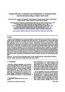
For the decoding problem over an FHMM, the above equation should be replaced by the fuzzy intersection in the numerator and fuzzy integral in the denominator. In both cases, the resulting posterior distribution is helpful to design K for the desired decoding accuracy. 2.4 Simulation study We simulate a plume source as independent particles following random walks which satisfy the advection and diffusion constraints. The model is reasonably accurate and the plume path generation is usually much faster than solving the advection-dispersion equation directly [18]. As an illustration, assuming Δt = 1s, the plume source is at (0, 0) with release rate 100 particles per second and duration of 8s. There are 20 sensors randomly deployed in a 1000×1000m2 field with sensing range of 50m for each sensor and at least 10 particles in its sensing area for a plume detection at any time. With wind velocity given by (vx(k), vy(k)) = (8, 5)m/s, longitudinal and transversal dispersivity L = 0.8, T = 0.2 and diffusion coefficient D = 0.9, one realization of the Gaussian plume at 100s is shown in Fig. 1 with two sensor detections.

Fig. 1. One realization of plume propagation at K = 100. We partition the region into 100 cells of the same square shape. It is assumed that initially there is no plume source in the sensing field. All 20 sensors are assumed to be synchronized and provide binary detections to a centralized data processor for plume mapping. The FHMM assumes pb = 0.005 and pc = 0.8. The plume source always starts at the bottom left cell at 4s with a constant release rate. Viterbi algorithm maintains all feasible solutions in its trellis graph while greedy heuristic algorithm only keeps the solutions within a Hamming distance of 8 to the initial candidate. We compare the probability of finding the correct cell and initial releasing time of the plume source after K time steps. The plume localization error probabilities are shown in Fig. 2 based on 5000 Monte Carlo runs for each K. We can

314

Advances in Greedy Algorithms

see that greedy heuristic algorithm has the localization error close to that using Viterbi algorithm and the performance gap decreases as K increases. Using Matlab to compile both algorithms on a Pentium 4 PC with 2.80GHz CPU, we found that the average time to find the best state sequence using greedy heuristic algorithm is 0.05s when K = 100 while Viterbi algorithm takes 5.3s in average to obtain the most likely sequence estimate. Thus the proposed greedy algorithm achieves the plume localization accuracy close to that using Viterbi algorithm while the computational time is orders faster than that using Viterbi algorithm. Our approach can also be used to estimate the total mass of plume release. However, there is no guarantee on its accuracy even for instantaneous release of a single plume due to the nature of binary sensor detection. To estimate the release rate sequence of a plume source, denser sensor coverage or more accurate plume concentration intensity measurement is needed. This problem will be addressed in the next section.

Fig. 2. Comparison of plume localization error probability with various observation length K.

3. Parameter estimation and model selection for gaussian plume sources This section deals with joint plume localization and release sequence estimation when the number of plume sources is unknown. We start with the plume source aggregation and sensor measurement model in Section 3.1. Section 3.2 presents the regularized least squares solution to the parameter estimation problem. Section 3.3 discusses the implementation of the joint model selection (on the number of sources) and parameter estimation using greedy algorithm and the choice of regularization parameter. Section 3.4 compares our approach with alternative regularization methods. Section 3.5 provides realistic source release scenarios to assess the performance of the proposed algorithm.

Greedy Methods in Plume Detection, Localization and Tracking

315

3.1 Plume aggregation and sensor measurement model We assume that the wind field in the search area can be accurately modeled and sensors can collect fairly accurate concentration readings in their neighboring areas. A Cartesian coordinate system is used with x-axis oriented towards the mean wind direction, y-axis in the cross-wind direction and z-axis in the vertical direction. If the source of a pollutant is located at (x0, y0, z0) with release rate q(t), then at time t, the concentration of the pollutant at some down-stream location (x, y, 0) can be written as [16] (19) where the kernel K(t, τ ) is (20) with mean wind speed u and diffusion coefficients Kx, Ky, Kz along x, y and z directions, respectively. We assume that there are J sensors deployed at fixed locations where sensor j is located at . Denote by c = {cj} the (xj, yj , 0) and collects N concentration readings cj = {C(xj , yj , 0, tn)} the discretized source release sequence collection of all sensor readings. Denote by q = {q(τi)} where q(τi) is the release rate at time τi. Ideally, we have the following observation equation (21) where p = (x0, y0, z0) denotes the unknown source location. Note that for measurement cj(xj , yj , 0, tn), the corresponding element a(jn,k) in A(p) is given by (22) where βnk is a quadrature weight [16, 17]. The estimation of source location p and release rate q can be formulated as the least squares problem given by (23) Note that this formulation is valid only for a single source. To extend the estimation problem to include multiple sources, we assume that the concentration readings are the results of aggregation from multiple source releases. Assume that there are s sources with unknown locations {p(i)} and release rate sequences {q(i)} . Then we have the following ideal observation equation (24) The source parameter estimation problem becomes identifying the number of sources, the corresponding origins and the release sequences jointly using only the concentration readings from multiple sensors.

316

Advances in Greedy Algorithms

3.2 Regularized least squares In the single source case, the matrix A in (23) can be analyzed for various source locations. By ranking the singular values of A, the authors of [16] found that the discrete time least squares problem (23) is in general ill-posed and suggested to use the Tikhonov regularization to ensure certain smoothness of q. However, for a source with an instantaneous release, the sequence q may have only a single spike, which violates the smoothness assumption. Nevertheless, for multiple sources with instantaneous releases, we will observe the aggregated sparse signal with an unknown number of spikes. In fact, the sparsity assumption is crucial for the identification of multiple sources with instantaneous releases at different times. To encourage the sparsity of the release rate sequence estimate, we propose to use lp-regularized least squares as the objective function, i.e., (25) where the regularization parameters p controls the sparsity of the solution q and λ makes the tradeoff between the goodness-of-fit to the observations and the complexity of the model. Note that p = 1 is popularly used in compressed sensing [10] due to its numerical reliability. In fact, for any given p, minimizing (25) becomes a convex program if one chooses p = 1. However, our l1-regularized least squares problem still requires non-convex optimization without knowing the source location p. In addition, when choosing the regularization term with 0 < p < 1, one favors a more sparse solution than that using l1regularization [7]. This might be helpful when one has prior knowledge about the type of release of plume sources. In this case, the regularization term &· & is not a norm, but d(x, y) = &x - y&

is still a metric.

When the concentration readings are the aggregation of individual release, we have to identify the number of sources and find their locations. In this case, we are facing a model selection problem, where model s corresponds to s sources with unknown locations and release rate sequences {q(i)} . Assuming that different sources have different {p(i)} instantaneous release times so that there is no identifiability issue among the models, we can choose model s that minimizes a modified version of (25)

(26) where (27) Note that the first term in the penalty encourages the sparsity of each identified source release sequence and the second term is for model complexity of the source location parameter based on the Bayesian information criterion [27]. The second term is necessary because one does not want to treat one source with two instantaneous releases (sparsity of 2) as two different sources with instantaneous releases at different time instances (sparsity of 1). In practice, when the locations of two sources are close, they could be identified as a

Greedy Methods in Plume Detection, Localization and Tracking

317

single source with aggregated release rate sequence. This seems to be acceptable when the locations of multiple sources are within the arrange of the localization accuracy obtained by minimizing (26). 3.3 Model selection and parameter estimation with a greedy algorithm Finding the optimal solution to (26) requires solving a high dimensional nonlinear optimization problem for any fixed regularization parameters p and λ. In practice, the number of sources is usually small and a strong source can have the dominant effect on the sensor readings. Thus it would be meaningful to identify and localize one source at a time by treating the impact from the remaining possible sources as additive noise. In this case, assuming the source location is given, one can obtain the sparse solution of the release rate sequence by solving the following optimization problem. (28) When p = 1, the problem becomes a convex program and is highly related to LASSO [29]. Once we obtain the release rate of the source, we can refine the estimate of source location by solving the regular nonlinear least squares problem given by (29) Note that for the newly estimated source location, the sparsity (non-zero locations) of the solution to (28) may change. We can iteratively update the release rate and source location estimate until the residual is comparable to the noise level of sensor readings. We can extend the above procedure to deal with unknown number of sources. We apply a greedy heuristic algorithm that iteratively refines the estimate of signal sparsity and the noise level to determine the appropriate regularization parameter. The algorithm is greedy in the sense of extracting one plume source at a time, from the strongest one to the weakest (based on the penalty term in the model selection criterion). It simultaneously determines the number of sources, the corresponding locations and release rate sequences by the following steps. 1. Set s = 1. 2. Initialization: Set k = 0, q(s)k = 0 with an initial guess of source location p(s)k. 3. Refining the estimate: Use Newton-Ralphson update (30) 4. 5.

to refine the estimated source release sequence. Choosing regularization parameter: Compute the median of the residual ⏐c - A(p(s)k)q(s)k+1⏐ and choose λ proportional to the estimated noise level. Denoising by soft thresholding: Compute the sparse approximation of q(s)k+1 by q(s) =T(q(s)k+1) where (31)

6.

Source localization: Solve the nonlinear least squares problem

318

Advances in Greedy Algorithms

(32) 7.

Model selection: Set k = k+1 and iterate until q(s) converges to a sparse solution q(s)* or a predetermined maximum number of iterations kmax has reached. Subtract out the identified source from sensor readings. (33) Repeat steps 2-6 until (34)

8.

Declare the number of sources (s - 1), the corresponding locations p(s - 1)* and release rate sequences q(s - 1)*. For any given λ and p(s)*, the above iterative procedure converges to the optimal solution of (28) for p = 1 [1]. We used the median estimator of the residue to obtain the noise level which is robust against outliers. It is less sensitive to possible model mismatch than using the mean of the residue when we initially assume that there is a single (strong) source which results in the concentration readings while treating other (weak) sources as noise. Note that the dimension of p(s) only depends on the model order, i.e., the number of sources, which is usually much lower than the dimension of release sequences q(s). Thus solving the nonlinear least squares problem (32) is less computationally demanding than solving (26) directly. When 0 < p < 1, (28) becomes non-convex program and any iterative procedure may be trapped at a local minimum. Another issue is that (24) may become underdetermined when A has rank deficiency. In such a case, the sparse solution to the following constrained optimization problem

is still meaningful. To encourage more sparsity of the release rate sequence with smaller p and solve the above constrained optimization problem directly, we apply iterative reweighted least squares (IRLS) update [7] and replace the soft thresholding step by (35) where the weighting matrix W(n) is diagonal with entries (36) The damping coefficient ε is chosen to be relatively large initially and decreases to a very small number when the above iteration is close to converge. Note that the IRLS algorithm converges in less than 100 iterations most of the time in our simulation study. Even though there is no theoretical guarantee that the resulting solution is globally optimal, we suspect that it does approach to near global minimum since the solution quality improves when using smaller p.

Greedy Methods in Plume Detection, Localization and Tracking

319

The above greedy algorithm can be interpreted as performing basis pursuit [13]. Specifically, given the stacked observation c, we want to find a good n term approximation using different sources as the basis functions from a general dictionary D. Denote by {gi} the i-th basis being selected. Basis pursuit proceeds as follows. 1. Initialization: • Approximation: s0 = 0 • Residual: r0 = c • Basis collection: Γ0 = φ 2. Pure greedy search:

Unfortunately, identifying a basis in the greedy pursuit is equivalent to localizing the origin of a single source, which requires solving a nonlinear least squares problem. The regularization on release rate sequence and penalty on the number of unknown sources prevent the resulting optimization problem from being ill-posed. Note that when the basis functions in the dictionary satisfy certain mutual incoherence property, the greedy basis pursuit algorithm guarantees finding the best n term approximation [13]. 3.4 Comparison with other regularization techniques Tikhonov's regularization has been proposed in [16, 17] which essentially uses the objective function (37) where L controls the smoothness of q(i) with the approximate form (38) The popular choice for obtaining a smooth solution is N = 2. Unfortunately, the above regularization technique only works for continuous releases from well separated sources. We rely on the sparsity of q(s) to identify the model order s, which is suitable for localizing multiple sources of instantaneous release type. Another sparsity enforced estimator was proposed in [4] which essentially minimizes the following objective function (39) For known source locations, the estimated release rate guarantees to recover all possible sparse signals with a large probability [4]. However, the above objective function is a nonsmooth function of p(s), which is difficult to optimize when both source locations and release rate sequences are unknown. In practice, we fix the source locations p(s) and solve

320

Advances in Greedy Algorithms

(39) via linear programming. Then we fix the release rate sequence q(s) and update p(s) in its gradient descent direction. The iteration continues until p(s) reaches a stationary solution and the sparsity of q(s) does not change. 3.5 Simulation of joint plume localization and release sequence estimation We present the simulation study of source localization and release rate estimation using multiple sensors. We are interested in both model selection and source parameter estimation accuracy. 3.5.1 Scenario generation Consider a single source located at (-40, 35, 12) with instantaneous release of q(10) = 2 · 105. We assume that the wind speed u = 1.8 along x-axis and Kx = Ky = 12, Kz = 0.2113. Five sensors, located at (0, 0), (15, 15), (30, 30), (45, 45), (60, 60), respectively, collect concentration readings synchronously with 100 samples per sensor. All sensors are on the ground with zero elevation. We add Gaussian noise to the sensor readings with standard deviation 4 · 10-3. Each sensor will have a plume detection when the concentration reading exceeds 0.01. Fig. 3 shows one realization of the concentration readings from the five sensors. We can see that sensor 1 has early detection while sensors 3-5 have relatively large peaks in the concentration readings. We also considered the case of two sources where one source located at (-40, 35, 12) has the instantaneous release of q(10)=2 · 105 and the other located at (-30, 15, 15) has the instantaneous release of q(50)=1 · 105. Fig. 4 shows one realization of the concentration readings from the five sensors. Compared with Fig. 3, we can barely see the effect of the second source release due to the detection delay and source aggregation. 3.5.2 Model selection and parameter estimation accuracy We want to compare our lp-regularization method with Tikhonov's method [16, 17] (denoted by p = 2) and Dantzig selector [4] (denoted by p = ∞) for both one-source and two-source cases. Note that Tikhonov's method is not appropriate for estimating instantaneous release rate, which is non-smooth. However, it is meaningful to study how the incorrect assumption in regularization may affect model selection accuracy. We estimated the probability of identifying the correct number of sources based on 100 realizations of each case. For those instances where the number of sources is correctly identified, we also computed the root mean square (RMS) error of the location estimate for each source. In the case of s = 2, the RMS error of the second source is in parentheses. The results are listed in Table 1. We can see that in the single source case, our lp-regularization method can identify the correct number of sources almost perfectly. In the two-source case, Tikhonov's method failed to identify the second source most of the time and Dantzig selector can only identify the correct number of sources with 64 out of 100 cases. Surprisingly, the proposed lpregularization method is able to find the correct model order with higher than 80% probability. As we reduce p, there is a slight increase in the probability of obtaining the correct number of sources due to the strong enforcement of sparsity. Among all cases where the first source is correctly identified, the root mean square error of the estimated release rate is 4.6 · 104 with p = 1. Note that the root mean square error of estimated location of the first source increases when we have a second source aggregated to it. Note also that the algorithm assuming the correct model order can only achieve the root mean square error of estimated location of the second source around 18 using lp-regularized method with p = 1.

Greedy Methods in Plume Detection, Localization and Tracking

321

These observations suggest that the lp-regularized least squares method is effective in joint model selection and parameter estimation for instantaneous source release.

Fig. 3. Sensor readings for a single source with instantaneous release.

Table 1. Comparison of Model Selection and Source Localization Accuracy with Different Regularization Methods 3.5.3 Model mismatch to continuous release source Consider a single source located at (-40, 35, 12) with continuous release rate

One realization of the concentration readings from the five sensors is shown in Fig. 5. Note that the concentration readings from sensors 2-5 have not reached their peaks by the end of the samples. This will in general make the source parameter estimation more difficult. In 100 realizations, the lp-regularized least squars method with p = 1 identified one source in 92 times and two sources in 8 times with their estimated locations close to each other. The incorrect identification of model order is due to the abrupt release at two time instances t = 10 and t = 50 with exponential decay of the release rate. The root mean square error of the estimated source location is 15.4 using the estimates from the correctly identified cases. Clearly, the lp-regularized least squares method can tolerate slight model mismatch when the release rate sequence is not overly sparse.

322

Advances in Greedy Algorithms

Fig. 4. Sensor readings for two sources, each with instantaneous release.

Fig. 5. Sensor readings for one source with continuous release.

4. Discussion and conclusions In this chapter, we studied plume detection, localization and tracking problem with two different settings. For plume mapping with binary detection sensors, we formulated the problem as finding the most likely state sequence based on a fuzzy hidden Markov model.

Greedy Methods in Plume Detection, Localization and Tracking

323

Under the assumption that each sensor has high detection and low false alarm probability, we proposed a greedy heuristic decoding algorithm with much less computational cost than the well known Viterbi algorithm. The plume localization accuracy of our algorithm is close to the optimal decoder using Viterbi algorithm when tracking a single plume using randomly deployed sensors. Our algorithm is applicable to general decoding problem over a long observation sequence when the localization error probability of the Viterbi decoder is small. There is a serious drawback of using FHMM for plume tracing. In our FHMM formulation, one can not distinguish whether a plume existence state is due to source releasing or plume propagation without knowing the whole state sequence. Thus one has to make tradeoff between the delay and localization accuracy. A refined plume propagation model based on more accurate sensor readings and contaminant transport physics was then used for source localization and release rate sequence estimation. When localizing unknown number of sources based on the observation of aggregated concentrations, we proposed an lpregularized least squares method to estimate the location and release rate of atmospheric pollution. For 0 ≤ p ≤ 1, the method enforces sparsity of the release sequence of each identified source. The proposed greedy method can identify multiple sources of instantaneous release type and can also localize sources of continuous release. The accuracy of source parameter estimation has been examined for the cases where the number of sources and the corresponding locations are unknown. In general, the least squares approach does not provide any measure of the estimation error. However, one can examine the residual and make additional assumptions such as additive Gaussian noise in order to quantify the covariance of the localization error. Through simulation study, we found that the proposed method is effective in localizing instantaneous release sources and has certain degree of tolerance to model mismatch. It is worth noting that the sensor locations, sampling rate and measurement accuracy can affect the source localization performance significantly. Finding the best sensor placement and sensing strategy in a given surveillance area is another important research theme and demands future work. We hope that with the advances in the development of greedy algorithms, many other challenging optimization tasks can be tackled with efficient and near optimal solutions.

5. References [1] S. Boyd, and L. Vandenberghe, Convex Optimization, Cambridge University Press, 2004. [2] S. M. Brennan, A. M. Mielke, and D. C. Torney, “Radiation Detection with Distributed Sensor Networks,” IEEE Computer, pp. 57-59, August 2004. [3] S. M. Brennan, A. M. Mielke, and D. C. Torney, “Radioactive Source Detection by Sensor Networks,” IEEE Nuclear Science, 52(3), pp. 813-819, 2005. [4] E. J. Candes and T. Tao,”The Dantzig Selector: Statistical Estimation When p Is Much Larger Than n,” submitted to Annals of Statistics, 2005. [5] T. H. Cormen, C. E. Leiserson, and R. L. Rivest, Introduction to Algorithms, first edition, MIT Press and McGraw-Hill, 1990. [6] T. M. Cover, and J. A. Thomas, Elements of Information Theory, New York: Wiley, 1991. [7] R. Chartrand, “Exact Reconstruction of Sparse Signals via Nonconvex Minimization,” IEEE Signal Processing Lett., 14, pp. 707-710, 2007. [8] J.-C. Chin, L.-H. Hou, J.-C. Hou, C. Ma, N.S. Rao, M. Saxena, M. Shankar, Y. Yong, and D.K.Y. Yau,”A Sensor-Cyber Network Testbed for Plume Detection, Identification, and Tracking,” 6th International Symposium on Information Processing in Sensor Networks, pp. 541-542, 2007.

324

Advances in Greedy Algorithms

[9] R. A. Dobbins, Atmospheric Motion and Air Pollution: An Introduction for Students of Engineering and Science, John Wiley & Sons, 1979. [10] D. L. Donoho, “Compressed Sensing,” IEEE Trans. Information Theory, 52, pp. 1289-1306, 2006. [11] J. A. Farrell, S. Pang, and W. Li, “Plume Mapping via Hidden Markov Methods," IEEE Trans. SMC-B, 33(6), pp. 850-863, 2003. [12] E. B. Fox, J. W. Fisher, and A. S. Willsky, “Detection and Localization of Material Releases with Sparse Sensor Configurations,” IEEE Trans. on Signal Processing, 55(5), pp. 1886-1898, May 2007. [13] P. S. Huggins, S. W. Zucker, “Greedy Basis Pursuit,”, IEEE Trans. Signal Processing, 55(7), pp. 3760-3772, July 2007. [14] H. Ishida, T. Nakamoto, T. Moriizumi, T. Kikas, and J. Janata, “Plume-Tracking Robots: A New Application of Chemical Sensors,”Biological Bulletin, 200, pp. 222-226, 2001. [15] H. Ishida, G. Nakayama, T. Nakamoto, and T. Moriizumi, “ Controlling A Gas/Odor Plume-Tracking Robot based on Transient Responses of Gas Sensors," IEEE Sensors Journal, 5(3), pp. 537-545, 2005. [16] P. Kathirgamanathan, R. McKibbin and R. I. McLachlan, “Source Release Rate Estimation of Atmospheric Pollution from Non-Steady Point Source - Part 1: Source at A Known Location,” Res. Lett. Inf. Math. Sci., 5, pp. 71-84, 2003. [17] P. Kathirgamanathan, R. McKibbin and R. I. McLachlan, “Source Release Rate Estimation of Atmospheric Pollution from Non-Steady Point Source - Part 2: Source at An Unknown Location,” Res. Lett. Inf. Math. Sci., 5, pp. 85-118, 2003. [18] C. Kennedy, H. Ericsson, and P. L. R. Wong, “Gaussian Plume Modeling of Contaminant Transport,” Stoch. Environ. Res. Risk Assess, 20, pp. 119-125, 2005. [19] J. Luo, “Low Complexity Maximum Likelihood Sequence Detection under High SNR,” submitted to IEEE Trans. Information Theory, Sept. 2006. [20] M. A. Mohamed, and P. Gader, “Generalized Hidden Markov Models - Part I: Theoretical Frameworks”, IEEE Trans. on Fuzzy Systems, 8(1), pp. 67-81, 2000. [21] M. A. Mohamed, and P. Gader, “Generalized Hidden Markov Models - Part II: Application to Handwritten Word Recognition", IEEE Trans. on Fuzzy Systems, 8(1), pp. 82-94, 2000. [22] A. Nehorai, B. Porat, and E. Paldi, “Detection and Localization of Vapor-Emitting Sources,”IEEE Transactions on Signal Processing, 43(1), pp. 243-253, 1995. [23] G. Nofsinger, and G. Cybenko, “Distributed Chemical Plume Process Detection,” IEEE MILCOM, Atlantic City, NJ, USA, 2005. [24] M. Ortner, and A. Nehorai, “A Sequential Detector for Biochemical Release in Realistic Environments,” IEEE Transactions on Signal Processing, 55(8), pp. 4173-4182, 2007. [25] L. R. Rabiner, “A Tutorial on Hidden Markov Models and Selected Applications in Speech Recognition,” Proc. of the IEEE, 77(2), pp. 257-286, 1989. [26] N. Rao, “Identification of Simple Product-Form Plumes Using Networks of Sensors With Random Errors,” Proc. Int. Conf. on Information Fusion, Florence, Italy, July 2006. [27] G. Schwartz, “Estimating the Dimension of a Model,” Annals of Statistics, vol.6, pp. 461-464, 1978. [28] J. N. Seinfeld and S. N. Pandis, Atmospheric Chemistry and Physics: From Air Pollution to Climate Change, John Wiley & Sons, New Jersey, 1997. [29] R. Tibshirani, “Regression Shrinkage and Selection via the LASSO," Journal Royal Statistical Society B, 58, pp. 267-288, 1996. [30] T. Zhao and A. Nehorai, ”Detecting and Estimating Biochemical Dispersion of A Moving Source in A Semi-Infinite Medium,” IEEE Transactions on Signal Processing, 54(6), pp. 2213-2225, 2006. [31] T. Zhao and A. Nehorai, “Distributed Sequential Bayesian Estimation of a Diffusive Source in Wireless Sensor Networks,", IEEE Transactions on Signal Processing, 55(4), pp. 1511-1524, 2007.