Green coverage detection on sub-orbital plantation images using anomaly detection Gabriel B. P. Costa and Moacir Ponti Instituto de Ciˆencias Matem´ aticas e de Computa¸ca ˜o — Universidade de S˜ ao Paulo 13566-590 S˜ ao Carlos, SP, Brazil
[email protected],
[email protected] http://www.icmc.usp.br/~moacir
Abstract. The green coverage region is a relevant information to be extracted from remote sensing agriculture images. Automatic methods based on threshold and vegetation indices are often applied to address this task. However, sub-orbital remote sensing images have elements that can hinder the automatic analysis. Also, supervised methods can suffer from imbalance since there is often many more green coverage samples available than regions of gaps, weed and degraded areas. We propose an anomaly detection approach to deal with these challenges. Parametric anomaly detection methods using the normal distribution were used and compared with vegetation indices, unsupervised and supervised learning methods. The results showed that anomaly detection algorithms can handle better the green coverage detection. The proposed methods showed similar or better accuracy when compared with the competing methods. It deals well with different images and with the imbalance problem, confirming the practical application of the approach. Keywords: Anomaly, outlier, remote sensing
1
Introduction
Precision agriculture can help small farmers in the management of plantations. One of the most important technologies in this context is remote sensing imagery. However satellite remote sensing can be expensive, while low-cost systems that acquire sub-orbital images can benefit developing countries and small properties[11]. A low-cost remote sensing system was proposed by Martins et al. [7] based on an image acquisition equipment attached to a balloon. This system acquires sub-orbital images that can be transmitted via radio frequency or processed offline. The advantages of this method includes the height control (often from 10 to 100 meters), the need of one or two persons to operate, and the low cost. The disadvantages are the limitation in regions with trees and electric wires, and a low load capability (from 2 to 4 kg). One of the most relevant information to be extracted from the image is the green coverage region. By accessing a map of green coverage it is possible to
2
Gabriel B. P. Costa and Moacir Ponti
locally adjust irrigation, application of fertilizers, and perform better weed control. To address this task, previous studies includes method based on threshold Otsu’s method, histograms and vegetation indices such as ExG (excess green) [4] among others. A combination of vegetation indices and mean-shift segmentation improved the previous results [9]. Sub-orbital images suffer from illumination variation, shadows and other elements that can hinder the automatic analysis. For this reason, when using tools of satellite remote sensing, it is often difficult to improve the results using only unsupervised methods such as those based on threshold and vegetation indices. Also, supervised methods can also not perform well since there is often many more green coverage samples available than regions of soil, weed, gaps and degraded areas. Besides, it can be a hard task to label many samples before using the system. In order to deal with these challenge, we propose an anomaly detection approach. Anomalies (or outliers, exceptions or deviations) are patterns with an unexpected behavior. Barnett and Lewis [1] defined anomaly as an observation (or subset of observations) which appears to be inconsistent with the remainder of that set of data. Due to the nature of the problem, anomalies are often rare and dealing with it can help on applications such as fault detection, fraud detection, network intrusion, etc. An anomaly detection (AD) method take as input a sample or set of samples, and identify whether those samples are “normal” or “abnormal”, according to what is expected to be found. On most applications the data is imbalanced, “normal” samples are widely available, while anomalies are scarce or not available [2]. The motivation to the application is that this approach needs mostly samples from normal data, that are abundant and easy to label, and few examples (and sometimes no examples) from anomalous data. We also organized a dataset based on sub-orbital images, available for download. Our contribution is to look at the green coverage detection as an anomaly detection process, so that green coverage will be considered normal behavior, while gaps, soil, degraded areas and others will be considered to be abnormal.
2
Low-Cost Remote Sensing System
A system built with a helium gas baloon model Skyhook Helikite was used to acquire the images. A digital camera with a 10 megapixel CCD sensor of size (1/2.3)-in was attached to the balloon with a radiofrequency controller board. It was build to provide an inexpensive solution for remote sensing in Brazil [7] [9]. For this study, a total of 12 images of plantations were obtained with an approximate height of 50 meters, from two different fields of common beans at 63 days after the emergence of the plants, in different days. The images were cropped to squared parcels, and resampled to 1024 × 1024 pixels, resulting in an approximate resolution of 3.1cm/pixel. The original images were acquired in RGB color model. Figure 1 shows versions of six images used in the experiments, converted to grayscale. The difference
Green coverage detection on plantation images using anomaly detection
3
between the two crops was the soil compaction, the second row of images were obtained from the crop with higher soil compaction. Due to the different weather conditions, there are images with different contrast and bright characteristics, and some of the images have motion blur due to the balloon movement.
Fig. 1. Examples of images obtained from two different crops of beans (first and second row of images with different soil compaction) using a low-cost remote sensing system.
2.1
Feature Extraction
In order to use the machine learning and anomaly detection methods, it is necessary to extract features from the image in order to build a feature vector. We selected a texture and a region-based color extractor. Haralick Texture Features : after converting the image to a grayscale version using the composition I = 0.2989 · R + 0.587 · G + 0.114 · B, the texture features were computed using 6 Haralick features [5] with a (0, 1) co-occurrence matrix: entropy, maximum probability, homogeneity, uniformity, contrast and correlation. CCV Color Features : the Color Coherence Vector method tries do codify how colors are organized in connected regions. It classifies each pixel as coherent or incoherent based on whether or not it is part of a large similarly-colored region [8]. The RGB image was quantized to 64 colors and a threshold of 25 was used to compute the CCV features.
4
3 3.1
Gabriel B. P. Costa and Moacir Ponti
Green coverage detection methods Vegetation Index
Vegetation index techniques uses arithmetic operations on the available bands (visible light, near-infrared, etc.). The aim is to to enhance some features, obtaining an image in which, for example, it is possible to visualize better the vegetation, with a better contrast between the response models in the available channels. These indices are often used in order to segment the green vegetation regions in agriculture remote sensing images. One of the most used ones, when only the visible light is available is the ExG, computed using ExG = 2G−R−B. After computing the index, a threshold method such as Otsu method is used to separate green coverage from other areas in the image, creating a binary image [9]. The user must interpret the results since the images can have zero or one values both for green coverage and without green coverage regions. 3.2
Unsupervised and supervised learning methods
Any machine learning method can be used to detect regions in remote sensing images. Unsupervised learning methods can separate pixels or sub-images in groups by using distances between them. In this case there is no previous knowledge involved, and the user must interpret the results given the output. Supervised learning methods are able to build a model for each class, e.g. green coverage and lack of green coverage. For this reason, it is important to have enough labeled data so that all every model is well built. In this study we use classic algorithms such as the k-Means, unsupervised method that minimizes the squared error with respect to samples and cluster centroids, and the Normal Bayes, a supervised probabilistic algorithm that assumes the data is normally distributed, but does not assumes independent features. We also investigated the Optimum-Path Forest classifier, a classifier based on graph theory, since it obtained good results on imbalanced datasets [10]. 3.3
Anomaly detection
In this paper we used methods that models only the normal data, using few abnormal samples in order to obtain a threshold for the detector. According to Hodge and Austing [6], the advantages of these methods are: a) needs mostly data labeled as normal and just a few labeled as abnormal, b) it is suitable for static or dynamic data, as it only learns one class, c) most method are incremental, d) it does not assume any distribution for the abnormal data. Three methods are proposed to the problem of detecting green coverage regions: the normal univariate and multivariate anomaly detectors [1], and our algorithm, based on the concatenation of features and detection in a normal parameter space [3].
Green coverage detection on plantation images using anomaly detection
5
– Normal univariate and multivariate detectors: uses the normal probability density function in order to learn with the normal data available. It can use a univariate model, defined in Equation 1, or a multivariate model, defined in Equation 2, that outputs the likelihood of a sample x belonging to the same law of the samples used to estimate the parameters of the distribution. 1 x−µ 2 1 p(x, µ, σ 2 ) = √ e− 2 ( σ ) . (1) σ 2π p(x, µ, Σ) =
1 (2π)n/2 |Σ|1/2
1
e− 2 (x−µ)
T
Σ −1 (x−µ)
.
(2)
The methods comprise three steps: 1. Estimate the normal distribution parameters: mean and standard deviation (univariate) or mean vector and covariance matrix (multivariate), using the data available, i.e. green coverage samples; 2. Find a threshold of anomaly detection: uses samples (normal and abnormal) from a validation set in order to find a threshold T for the likelihood p that maximizes the accuracy value. 3. Detection: compute its likelihood using the estimated parameters, if the value is lower than T it is considered an anomaly. – Parameter space anomaly detector: selects randomly from the training set M pairs of samples. Concatenates all features of each pair of normal samples, and computes mean and standard deviation for the whole concatenated vector. Each concatenated pair is a point in a parameter space θ = (µ, σ) ∈ × + , forming a point cloud, from which a convex hull is computed. This convex hull captures the normal behaviour. The algorithm tries to detect abnormal samples by concatenating them with normal samples and observing the deviation from the normal point cloud convex hull. The method comprises the following steps [3]: 1. Select pairs of normal instances, e.g. a and b, concatenate the features of a and b, and estimate the parameters µ and σ for each pair, 2. Compute a convex hull HN from the 2D point cloud. 3. Find a threshold of anomaly detection: uses samples (normal and abnormal) from a validation set in order to find a threshold P that maximizes the accuracy value for the perturbation caused by concatenating normal with abnormal samples, forming a new convex hull HT . The perturbation is the distance of the created point to all points in the convex hull computer in the previous step. 4. Detection: concatenate each point that contributed to the convex hull HN with the unknown pattern x. Estimate the parameters µ and σ and compute a new convex hull HT . If the intersection of HT and HN is lower than P , consider it an anomaly. This method captures data similarly to the normal univariate method. However it has more potential to be incremental, since new samples can be added in the normal point cloud in constant time.
R R
6
Gabriel B. P. Costa and Moacir Ponti
4
Experiments
All images were manually labeled by three agronomists. These specialists segmented the images in two disjunct regions: i) green coverage and ii) vegetation gaps, soil, degraded areas and others. The agreement between the specialists was of 91.7%±5.2. The images labeled by the agronomist with the higher interagreement was used as ground truth. For the classic vegetation index methods, each image pixel was used to detect green coverage since these methods need the whole image to process. In the other hand, sub-images of 100 × 100 pixels, also labeled by the agronomists, are used as observations for the other methods. The use of sub-images is feasible because the resolution is high when compared with satellite images. This high resolution is possible because the images were acquired by a sub-orbital equipment at just 50 meters as described in section 2. The six Haralick descriptors and the CCV feature vector, described in section 2.1, were computed for each one of the 230 sub-images. The dataset anomaly rate, i.e., the proportion of not normal samples, is ∼ 9%. The parameters for the CCV methods were found experimentally, after testing on a separate validation set of 20 images. The settings for each methods used to detect green coverage are: – Unsupervised methods: • Excess Green (ExG) and Mean-shift with Excess Green (MS-ExG): computed in the whole image, using each pixel as observation; • k-Means: computed using each feature vector extracted from the subimages as an observation. – Supervised learning methods: computed using each feature vector extracted from the sub-images as an observation. Uses 70% of both normal and abnormal samples for training, and 30% for testing. • Normal Bayes and Optimum-path Forest (OPF). – Anomaly detection (AD) methods: computed using each feature vector extracted from the sub-images as an observation. Uses 55% of normal samples for training, %15 of both normal and abnormal samples for validation, and 30% for testing. • Normal univariate, normal multivariate and parameter space AD. 4.1
Evaluation
We used a repeated random sub-sampling validation, each experiment was repeated 100 times. The average and standard deviation were computed by these repetitions. The evaluation was based on the balanced accuracy value that takes into account the balance between the classes: Pc [ei,1 + ei,2 ] F P (i) F N (i) , ei,1 = , ei,2 = , i = 1, ..., c, Acc = 1 − i=1 2c N − N (i) N (i) where c is the number of classes, ei,1 + ei,2 ] is the partial error of the class i, F N (i) (false negatives) is the number of samples belonging to i incorrectly classified as belonging to other classes, and F P (i) (false positives) the samples j 6= i that were assigned to i [9].
Green coverage detection on plantation images using anomaly detection
5
7
Results and Discussion
The average accuracies (in percentages) for each method are presented in Table 1. The anomaly detection methods showed accuracies similar or better than the best previously proposed methods. Threshold methods used the ExG index, while the learning methods used texture or color features. The results shows that texture features have better discriminative potential when compared to the color features for this application. Table 1. Average accuracy and standard deviation for the investigated methods.
Threshold Methods ExG 76.5±8.1 — MS+ExG 81.1±7.3 — Learning Methods Haralick-8 CCV-64 k-Means 66.0±9.0 59.7±4.7 Normal Bayes 68.7±9.5 62.2±10.2 OPF 60.7±3.7 64.3±13.0 Parameter space AD 79.1±9.1 69.5±9.5 Normal Univariate AD 77.9±8.9 68.7±9.1 Normal Multivariate AD 89.7±6.9 70.1±6.8
The unsupervised methods based on vegetation indices, including the recently published MS-ExG, performed well, with results comparable with the proposed methods: parameter space AD and normal univariate AD. However, it is important to note that the unsupervised results must be interpreted after the algorithm outputs the processed image, while the anomaly detection algorithms already have a meaningful output. Due to the scarce anomaly data available, the supervised learning methods (classifiers) produced mediocre results. The clustering algorithm, that used feature vectors to produce the results, performed worst than those based on vegetation indices. It is probably because the ExG and MS-ExG methods used each pixel value as an observation, while the k-Means used the feature vector computed over the 100×100 pixel sub-images.
6
Conclusions
This paper reports results of an anomaly detection methods applied to the green coverage detection problem. The main reasons for the success of this strategy is that: it does not assume any given distribution of the abnormal data, and does
8
Gabriel B. P. Costa and Moacir Ponti
not require much abnormal samples to be trained. Besides, this approach carries most advantages of partially supervised algorithms, such as the incremental capability, in which new samples can be easily added to the model. Whilst the multivariate method obtained the best result, the other methods showed good potential in this application. Future works can explore variations of the proposed parameter space, including multiple parameters that can capture correlations, exploring the use of the anomalous data in the training step, and improving the feature fusion, presently carried out by concatenation. The experimental evidence showed that the green coverage detection can be successfully treated as an anomaly detection problem, benefiting applications in precision agriculture that uses low-cost sub-orbital images.
Acknowledgment This work was supported by FAPESP (grants n.11/16411-4 and n.12/12524-1).
References 1. Barnett, V., Lewis, T.: Outliers in statistical data. John Wiley & Sons (1994) 2. Chandola, V., Banerjee, A., Kumar, A.: Anomaly detection: a survey. ACM Computing Surveys 41(3), 15 (2009) 3. Costa, G., Ponti, M., Frery, A.: Partially supervised anomaly detection using convex hulls on a 2D parameter space. In: Partially Supervised Learning. LNAI, vol. 8183, pp. 1–8 (2013) 4. G´ee, C., Bossu, J., Jones, G., Truchetet: Crop/weed discrimination in perspective agronomic images. Comput. Electron. Agr. 62, 49–59 (2008) 5. Haralick, R., Shanmugan, K., Dinstein, I.: Textural features for image classification. IEEE Transactions on Systems, Man and Cybernetics SMC-3(6), 610–621 (1973) 6. Hodge, V.J., Austin, J.: A survey of outlier detection methodologies. Artificial Intelligence Review 22(2), 85–126 (2004) 7. Martins, F.C.M.: Evaluation of compact areas in the bean culture using remote sensing techniques (in portuguese). Master’s thesis, UFV, MG, Brazil (2010) 8. Pass, G., Zabih, R., Miller, J.: Comparing images using color coherence vectors. In: ACM Multimedia 96. pp. 65–73 (1996) 9. Ponti, M.P.: Segmentation of low-cost remote sensing images combining vegetation indices and mean shift. Geoscience and Remote Sensing Letters, IEEE 10(1), 67–70 (2013) 10. Ponti-Jr., M.P., Papa, J.P., Levada, A.L.M.: A Markov Random Field model for combining Optimum-Path Forest classifiers using decision graphs and Game Strategy Approach. In: Progress in Pattern Recognition, Image Analysis, Computer Vision, and Applications (CIARP 2011). LNCS, vol. 7042, pp. 581–590 (2011) 11. Swain, K., Thomson, S., Jayasuriya, H.: Adoption of an unmanned helicopter for low-altitude remote sensing to estimate yield and total biomass of a rice crop. Transactions of the ASABE 53(1), 21–27 (2010)