Theory and Applications of Mathematics & Computer Science 3 (1) (2013) 13–31
Unsupervised Detection of Outlier Images Using Multi-Order Image Transforms Lior Shamira,∗ a
Lawrence Technological University, 21000 W Ten Mile Rd., Southfield, MI 48075, United States.
Abstract The task of unsupervised detection of peculiar images has immediate applications to numerous scientific disciplines such as astronomy and biology. Here we describe a simple non-parametric method that uses multi-order image transforms for the purpose of automatic unsupervised detection of peculiar images in image datasets. The method is based on computing a large set of image features from the raw pixels and the first and second order of several combinations of image transforms. Then, the features are assigned weights based on their variance, and the peculiarity of each image is determined by its weighted Euclidean distance from the centroid such that the weights are computed from the variance. Experimental results show that features extracted from multi-order image transforms can be used to automatically detect peculiar images in an unsupervised fashion in different image datasets, including faces, paintings, microscopy images, and more, and can be used to find uncommon or peculiar images in large datasets in cases where the target image of interest is not known. The performance of the method is superior to general methods such as one-class SVM. Source code and data used in this paper are publicly available, and can be used as a benchmark to develop and compare the performance of algorithms for unsupervised detection of peculiar images.
Keywords: Outlier detection, peculiar images, image analysis, image transform, multi-order transforms. 2010 MSC: 68T10, 62H35, 68T45, 62H30 .
1. Introduction Unsupervised detection of peculiar images is the ability of a computer system to automatically detect images that are different from the other “regular” images in an image dataset. While in tasks such as image classification the system can be trained in a supervised fashion using “ground truth” samples, in unsupervised detection of peculiar images the algorithm cannot rely on data samples or models that reflect the “regular” images or the target images of interest. The problem of detecting data points significantly different from the other data is often referred to as outlier detection (Hodge & Austin, 2004). Many established algorithms consider outlier ∗
Corresponding author Email address:
[email protected] (Lior Shamir)
14
Lior Shamir / Theory and Applications of Mathematics & Computer Science 3 (1) (2013) 13–31
detection as a by-product of clustering algorithms by searching for background noise samples that do not belong in a cluster (Aggarwal & Yu, 2000; Guha, Rastogi & Shim, 2001). Other methods are based on searching for samples that do not belong in a cluster and are also not background noise, but are substantially different from the other samples in the dataset (Breunig et al., 2000; Knorr & Ng, 1999; Fan et al., 2006). While many of the outlier detection algorithms were designed and tested using lower dimensionality, other methods aim at automatic outlier detection in higher dimensionality data (Aggarwal & Yu, 2001; Roth, 2005; Fan, Cehn & Lin, 2005; Lukashevich, Nowak & Dunker, 2009). Applications of outlier detection include credit card fraud, network intrusion detection, surveillance, financial applications, cell phone fraud, safety critical systems, loan application processing, defect detection in factory production lines, and sensor networks (Zhang et al., 2007). While outlier detection has been studied in the context of a broad range of applications, less work has yet been done on unsupervised detection of peculiar images in image datasets. Here we describe a generic method that can be used for automatic detection of peculiar images in image datasets based on a large set of image content descriptors extracted from the raw pixels, image transforms, and compound image transforms. Applications include, for instance, the search for peculiar cells or tissues in large datasets of microscope images, which can be used to detect phenotypes of particular scientific interest (d‘Onofrio & Mango, 1984; Carpenter, 2007; Jonesa et al., 2009). When the target image is known, the task of detecting a peculiar image can be related to the problem of Content-Based Image Retrieval, and numerous effective methods of measuring similarities between images in the context of CBIR have been proposed (Bilenko, Basu, & Mooney, 2004; Kameyama et al., 2006). However, since in this study the detection of a peculiar image in an image dataset should be done automatically in an unsupervised manner, no assumptions can be made neither about the target image nor about the context of the images in the data base. That is, the computer system should automatically characterize the “typical” image in the dataset, and detect images that are different from it. Since no pre-defined model of the data can be used, effective systems for unsupervised automatic detection of peculiar images need to extract different image features that will cover different aspects of the image content, and thus be able to characterize and analyze a broad spectrum of image data. Here we use a large set of image content descriptors extracted from the raw images, image transforms, and multi-order transforms, and apply a statistical analysis to weight the different image features by their ability to reflect the data and detect peculiar images. The primary advantage of the method is its generality, which makes it effective for the analysis of a broad variety of image datasets without the need for tuning or adjustments. In Section 2 we briefly describe the set of image features and multi-order transform model used in this study, in Section 3 we describe the unsupervised detection of the peculiar images, in Section 4 the performance evaluation method of the proposed algorithm is discussed, and in Section 5 the experimental results are presented. 2. Image features The set of image content descriptors used in this study is based on the feature set used by the wndchrm algorithm, which is a large set of numerical image content descriptors that cover a broad
Lior Shamir / Theory and Applications of Mathematics & Computer Science 3 (1) (2013) 13–31
15
range of aspects of the visual content (Shamir et al., 2008a; Orlov et al., 2008; Shamir et al., 2010). Basically, the wndchrm feature set includes several generic image features such as high-contrast features (object statistics, edge statistics, Gabor filters), textures (Haralick, Tamura), statistical distribution of the pixel values (multi-scale histograms, first four moments), factors from polynomial decomposition of the image (Chebyshev statistics, Chebyshev-Fourier statistics, Zernike polynomials), Radon features, and fractal features. A detailed description of these image content descriptors and the way they are used in the context of the wndchrm feature set is available in (Shamir et al., 2008a; Orlov et al., 2008; Shamir et al., 2010; Shamir, 2008; Shamir et al., 2009). The reason for using a large set of features is that the search for peculiar images is unsupervised, and no assumptions can be made regarding the possible difference between the peculiar and non-peculiar images. Therefore, it is important that the set of image content descriptors is comprehensive enough so that at least some of the image features will be likely to sense differences between a regular and a peculiar image in a given image dataset. As will be discussed in Section 5, a key contributor to the ability of the method proposed in this paper to detect peculiar images in an unsupervised fashion is the extraction of the image content descriptors not just from the raw pixels, but also from image transforms and compound image transforms. The extraction of image features from compound image transforms has been shown to contribute significantly to the performance of general-purpose image classifiers (Shamir et al., 2008a; Orlov et al., 2008; Shamir et al., 2010, 2009), and can therefore be effective for peculiar image detection in cases where the differences between the typical and the peculiar image should be determined automatically, without using “ground truth” samples or any other prior knowledge about the data. The image transforms include the Fourier, Chebyshev, Wavelet, and the edge-magnitude transform, as well as multi-order transform combinations. The combinations of transforms include the Fourier transform of the Chebyshev transform, the wavelet transform of the Chebyshev transform, the Fourier transform of the wavelet transform, the wavelet transform of the Fourier transform, the Chebyshev transform of the Fourier transform, and the Fourier and Chebyshev transforms of the edge magnitude transform. A detailed description of the tandem transform combinations can be found in (Shamir et al., 2010; Shamir, 2008), and the total number of images features extracted using these transforms is 2659 (Shamir et al., 2008a; Shamir, 2008). The length of the chain of transforms is limited to the first and second order of the image transforms, as experiments showed that using compound transforms with order higher than two typically does not contribute to the informativeness of the image analysis system (Shamir et al., 2009). The effect of using the multi-order image transforms on the ability of the algorithm to automatically detect peculiar images will be discussed in Section 5. For color images we used a color transform, which is based on transforming the RGB pixels into the HSV space, followed by classification of the HSV triplets into one of 16 color classes using fuzzy logic modeling of the human perception of these colors (Shamir et al., 2006). Then, the Fourier, Chebyshev, and wavelet transforms of the color transform are computed, and the set of image features is extracted as described in (Shamir et al., 2010). When the color transform is also used, the total number of image features is 3658 (Shamir et al., 2010). Figure 1 illustrates the paths of the transforms and compound transforms used by the feature set.
16
Lior Shamir / Theory and Applications of Mathematics & Computer Science 3 (1) (2013) 13–31
Figure 1. Paths of multi-order image transforms.
3. Automatic detection of peculiar images In order to automatically detect peculiar images, it is first required to characterize the “typical” image in the dataset. Since many image features are used without prior knowledge about the dataset, it can be assumed that not all content descriptors are relevant to the image dataset at hand, and might represent noise. Therefore, it is required to select the image features that are the most informative, and can potentially discriminate between peculiar and non-peculiar images. In the first stage of the algorithm, all image features are normalized to the interval [0, 1], so that the differences between the values of different image features can be compared without introducing a numerical bias. For instance, if the values of one image feature are in the range of [0, 1000] while the values of another are in the range of [0, 10], a numerical difference of 5 between the values of the first feature extracted from two different images can be considered small, while the same numerical difference can be much more substantial for the second feature, in which it is half of the entire range. In the next step, the mean, median, and variance of each image feature are computed. To characterize the “typical” feature values of an image in the dataset, the highest 5% and the lowest 5% of the values of each image feature are ignored when computing the mean and standard deviation, so that extreme values that results from noise, artifacts, or peculiar images will not affect the mean and variance of the “typical” images. After these values are computed, each image in the dataset is compared to the “typical” image using Equation 3.1 Di =
X | fi − f | , (1 − σ f )k · σ f f ∈F
(3.1)
where Di is the dissimilarity value of image i from the “typical” image in the dataset, f is a feature in the feature set F, f is the median of the values of feature f in the given image dataset, fi is the value of the feature f computed from the image i, σ f is the standard deviation of feature f, and k is a constant value set to 25. The value of k will be thoroughly discussed in Section 5. The Di dissimilarity value can be conceptualized as the sum of Z scores computed for each feature separately, such that each score‘s contribution to the total distance is inversely dependent on
Lior Shamir / Theory and Applications of Mathematics & Computer Science 3 (1) (2013) 13–31
17
the standard deviation. That is, features that have lower standard deviation are considered more “representative” features, while feature that their values are more sparsely distributed are assumed to provide a weaker representation of the “typical” image and are therefore assigned with a lower score and have a weaker affect on the dissimilarity value. Clearly, image features that their values are constant across the dataset (and therefore σ = 0) cannot provide any useful information in this model, and can therefore be safely ignored without affecting the performance. On the other hand, the values of some of the other features can be sparsely distributed across the image dataset, and therefore the median of these values cannot be considered as a value that reliably represents the typical image. For that reason, the effect of each image feature is weighted by its standard deviation, which is used as an assessment of the feature‘s informativeness and its ability to characterize the typical image. While in Equation 3.1 the effect of features that their values are sparsely distributed is weakened by using the standard deviation as a measurement of their informativeness, it can be assumed that many of the features will not be informative for a given image dataset at hand, and therefore the high number of irrelevant features can add noise to the analysis and negatively affect the performance. In order to reduce the effect of non-informative features, 90% of the features with the highest σ are ignored, and the remaining 10% are used by Equation 3.1 to compute the distance between a given image and the “typical” image in the dataset. Since the image features are also weighted by their standard deviation, the performance of this method is not highly sensitive to small changes in the number of features that are used, as will be discussed in Section 5. This approach of combining feature selection and feature weighting is conceptually similar to the approach of the feature selection in the wndchrm image classifier (Shamir et al., 2008a; Orlov et al., 2008; Shamir et al., 2010). In many cases, using σ to assess the informativeness of the features and their ability to differentiate between a peculiar and a typical image might not be optimal and can lead to the sacrifice of some of the information. For instance, if the values of a certain image feature range between 0 and 0.8 for most images in the dataset, but is always 1 for a certain peculiar image, this feature could have been effectively used to detect the peculiar image, but will be assigned with a low score due to the sparse distribution of the values. On the other hand, features can be assigned with high scores due to the consistency of their values, while these image features might have little ability to differentiate between a typical and a peculiar image. Since the goal of the method described in this paper is to detect peculiar images in an unsupervised fashion, no assumptions or prior knowledge about the data can be used, and therefore the image content descriptors cannot be selected or scored based on a target peculiar image. However, by using a large set of image features, it can be expected that some of the features that are assigned with high scores will be able to differentiate between a peculiar and a typical image. This will be demonstrated in Section 5. In summary, the following pseudo code summarizes the outlier detection algorithm: Step 1: Compute image features for all images. Step 2: Reject the lowest and highest 5% values of each feature. Step 3: Compute the mean M f of the values of each feature f.
18
Lior Shamir / Theory and Applications of Mathematics & Computer Science 3 (1) (2013) 13–31
Step 4: Compute the σ f of the values of each feature f. Step 5: Reject 90% of the features with the lowest σ. qP k Step 6: Compute d for each image I such that d = f (1 − σ f ) ·
(I f −M f ) . σf
Step 7: Sort the images in the dataset by d. The computational complexity of the algorithm is O(F · I log I), where I is the number of images and F is the number of features computed for each image. The computational complexity is determined by the complexity of sorting all values of each feature, which is the most computationally demanding task in the algorithm described above. The bottleneck of the process, however, is the computational complexity of the Wndchrm feature set, which is much more complex as described in (Shamir et al., 2008a, 2009). 4. Performance evaluation In order to test the performance of the proposed method, several different image datasets were used. These datasets include the Brodatz texture album (Brodatz, 1966), the COIL-20 object image collection (Nene, Nayar & Murase, 1996), JAFFE and AT&T face datasets (Samaria & Harter, 1994; Lynos et al., 1998), the MNIST handwritten digit collection (LeCun et al., 1998; Liu et al., 2003), and a dataset of digitized paintings of Van Gogh, Monet, Dali, and Pollock Shamir et al. (2010). Since the MNIST dataset contains a large number of images, a subset of 100 images from the first two classes (0 and 1) were used in the experiment. For microscopy images we used the CHO (Chinese Hamster Ovary) dataset (Boland & Murphy, 2001), consisting of fluorescence 512×382 microscopy images of different sub-cellular compartments, and the Pollen dataset (Duller et al., 1999), which is a dataset of 25×25 images of geometric features of pollen grains. The CHO dataset might not be considered a perfect representation of biological content (Shamir et al., 2011), but it is used in this study for general-purpose outlier detection. These two datasets are available for download as part of the IICBU-2008 benchmark suite at http: //ome.grc.nia.nih.gov/iicbu2008 (Shamir et al., 2008b), and sample images of the different classes are shown by Figures 2 and 3. The image datasets used in this study are listed in Table 1.
Figure 2. Sample images of class “obj 198” (top) and “obj 212” (bottom) taken from the pollen dataset.
Lior Shamir / Theory and Applications of Mathematics & Computer Science 3 (1) (2013) 13–31
19
Table 1. Image datasets used for the experiments.
dataset Pollen CHO JAFFE AT&T Painters 1 Painters 2 Brodatz 1 Brodatz 2 MNIST COIL-20
typical class obj 198 giantin KA 1 Pollock Monet Bark Wood 0 obj1
peculiar class obj 212 hoechst KL 2 Dali Van Gogh Brick Wool 1 obj2
images per class 45 69 22 10 30 30 4 4 100 71
Figure 3. Sample images of giantin (left) and hoechst (right) taken from the CHO dataset.
As the table shows, these datasets were used such that two classes from each dataset were selected: one class was used as the “typical” class and the other as a pool of “peculiar” images.
20
Lior Shamir / Theory and Applications of Mathematics & Computer Science 3 (1) (2013) 13–31
In each run the tested dataset included all images from the typical class, and one image from the peculiar class. The experiment was repeated for each image in the peculiar class, such that in each run a different image from the peculiar class served as the peculiar image. For instance, the AT&T face dataset has 10 images in each class, and therefore it was tested 10 times such that in each run all 10 images of person 1 were used and one image of person 2 (a different image in each of the 10 runs). The goal of the algorithm was to automatically detect the single image of person 2 among the dataset of 11 images (10 images of person 1 and one image of person 2). The performance was evaluated by the number of times the algorithm correctly detected the peculiar image in the set (which included the “typical” images and the one “peculiar” image), divided by the total number of images in the peculiar class. Another performance metrics used in this study is the rank-10 detection accuracy, which was measured as the percentage of the cases in which the peculiar image was among the first 10 candidates with the highest dissimilarity value as determined by Equation 3.1. 5. Results The performance of the automatic detection of peculiar images was evaluated as described in Section 4, and the rank-1 and rank-10 detection accuracies for each of the tested datasets are listed in Table 2. Table 2. Rank-1 and rank-10 accuracy of the detection of the peculiar image.
Dataset Pollen CHO Jaffe AT&T Painters 1 Painters 2 Brodatz 1 Brodatz 2 MNIST COIL-20
Rank-1 accuracy 29/45 57/69 16/22 10/10 26/30 0/30 4/4 4/4 29/100 38/71
Rank-10 accuracy 34/45 69/69 22/22 10/10 30/30 18/30 4/4 4/4 92/100 71/71
As the table shows, in almost all cases the proposed algorithm was able to automatically detect the peculiar images in accuracy significantly better than random. For instance, with the Pollen dataset the algorithm was able to automatically find the peculiar image in 29 times out of 45 attempts (each attempt with a different image), and the rank-10 detection was accurate in 34 times. The noticeable exception is the second datasets of painters, which consists of paintings of Monet and Van Gogh. In that case, the proposed method was not able to automatically detect any of the tested Van Gogh paintings in a set of Monet paintings, and the rank-10 accuracy was 60%. Since Monet and Van Gogh were inspired from each other, their artistic styles are similar to each other, and it usually requires knowledge in art to differentiate between the works of the two painters.
Lior Shamir / Theory and Applications of Mathematics & Computer Science 3 (1) (2013) 13–31
21
The other painter dataset that was tested demonstrated a much higher detection accuracy since the two painters, Jackson Pollock and Salvador Dali, belong in different schools of art (Abstract Expressionism and Surrealism, respectively) and the differences between their styles are highly noticeable even without any previous knowledge or training in art. The results specified in Table 2 demonstrate the generality of the method and its ability to handle very different image datasets in a fully automatic fashion, and without the need to select or tune parameters. The generality of the method can also be demonstrated by the different classes of the Pollen dataset. While the results in Table 2 are based on obj 198 as the “typical” class and “obj 212” as the peculiar class, the pollen dataset includes seven classes (Shamir et al., 2008b). Table 3 shows the rank-1 detection accuracy of all combinations of the seven classes in the pollen dataset, such that each cell is the detection accuracy when the row the “typical” class and the column is the “peculiar” class. As the table shows, the detection accuracy is significantly higher than random in all combinations of “typical” and “peculiar” classes, demonstrating the generality of the proposed method. Table 3. Rank-1 detection accuracy (%) of all combinations of typical and peculiar classes using the pollen dataset.
Regular\Peculiar 198 212 216 360 361 405 406
198 55 63 61 57 66 63
212 64 67 64 67 71 59
216 51 55 67 65 73 65
360 67 65 63 67 69 69
361 53 58 58 64 67 69
405 69 67 64 72 72 61
406 67 67 64 69 69 71 -
As discussed in Section 3, 90% of the image features with the highest σ are ignored. Changing the number of features that are rejected and not used by the image dissimilarity evaluation of Equation 3.1 can change the dissimilarity value determined by the Equation for each image, and consequently affect the performance of the algorithm. Figures 4 and 5 show the rank-1 and rank-10 detection accuracy of the peculiar images when the number of used features is changed. As the graphs show, while the peculiar image detection accuracy of some image datasets peaks when 10% of the features are used, in other datasets such as MNIST or COIL-20 the detection accuracy peaks when 40% of the features are used. In the case of MNIST, the rank-1 detection accuracy was elevated from 29% when 10% of the features were used to 94% with 40% of the image features. This shows that the detection of peculiar images can be optimized if the number of used image features is adjusted for the specific dataset. However, since the detection of the peculiar image is unsupervised, and in many cases the target peculiar image is unknown, adjusting the parameters for optimizing the performance based on sample target peculiar images might not be possible, and it is therefore required to use a general pre-defined parameter setting as was done for the performance figures reported in Table 2. Another value that was determined experimentally is the K values in Equation 3.1. Figures 6
22
Lior Shamir / Theory and Applications of Mathematics & Computer Science 3 (1) (2013) 13–31 100 90 80 Pollen CHO Jaffe AT&T Painters 1 Painters 2 Brodatz 1 Brodatz 2 MNIST COIL-20
70 60 50 40 30 20 10 0 0
0.1
0.2
0.3
0.4
0.5
Features used
Figure 4. The rank-1 detection accuracy of the peculiar image as a function of the amount of features used.
and 7 show the rank-1 and rank-10 detection accuracy of the peculiar image as a function of the value of this parameter. In all cases, 10% of the image content descriptors were used as described in Section 3. As the graphs show, the detection accuracy of the CHO dataset drops as the value of K increases, and the detection of a Dali painting in a set of Jackson Pollock paintings also peaks when the value of K is low. However, in most cases the detection accuracy of the peculiar image reaches its maximum when the value of K is around 25. In some of the tested image datasets, such as the Brodatz texture datasets and the rank-10 of the Painters 1 and COIL-20 datasets, the detection accuracy of the peculiar image remained perfect regardless of the value of K. A single peculiar image is expected to be detected more easily among a smaller dataset of regular images. That is, finding a peculiar image hidden in a dataset of millions of images is expected to be a more difficult task than finding a peculiar image in a dataset of just a dozen regular images. On the other hand, the presence of a large number of regular images allows the algorithm to find the image features that can discriminate between peculiar and regular images, and better estimate the weights of the features by their informativeness and ability to discriminate between a regular and a peculiar image as described in Section 3. To study the effect of the number of the regular images in the dataset we used the MNIST dataset, which provides a sufficient number of images of handwritten digits “0” and “1”. Figure 8 shows the rank-1 and rank-10 detection accuracy of a peculiar image when changing the number of regular images in the dataset using 1000 images of the handwritten digit “0”. As the graph shows, the detection accuracy generally drops as more regular images are added
Lior Shamir / Theory and Applications of Mathematics & Computer Science 3 (1) (2013) 13–31
23
100 90 80 Pollen CHO Jaffe AT&T Painters 1 Painters 2 Brodatz 1 Brodatz 2 MNIST COIL-20
70 60 50 40 30 20 10 0 0
0.1
0.2
0.3
0.4
0.5
Features used
Figure 5. The rank-10 detection accuracy of the peculiar image as a function of the amount of features used.
to the dataset. Clearly, this is due to the lower difficulty of finding a peculiar image in a dataset of 50 images compared to correctly finding a single peculiar image among a dataset of 1000 regular images. However, while the rank-10 accuracy decreases as the number of regular images gets higher, the rank-1 detection accuracy drops to ∼30% at around 80 regular images, but marginally changes when more regular images are added to the dataset. This can be due to the effect of the better weights assigned to the image features when the number of non-peculiar images in the dataset increases, which improve the ability of the algorithm to characterize the “typical” image in the dataset and differentiate it from peculiar images. It should be noted, however, that while a higher number of regular images improves the feature weights, it also increases the probability that one the regular images in the dataset will be assigned with a high dissimilarity value computed by Equation 3.1. Since the algorithm aims to detect the irregular images in an unsupervised fashion, any difference between one of the images in the dataset and the “typical” image might lead to the detection of that image as “peculiar”. For instance, in the MNIST dataset of the handwritten digit “0” the 10 most common images that were detected by the proposed algorithm as peculiar are shown in Figure 9. As the figure shows, some of these handwritten digits are noticeably different from a standard handwritten digit “0”. For instance, the top left digit has a black dot near it, while other images of handwritten “0” feature incomplete circles or thick lines. These images can confuse the algorithm since they are different from the typical image of the digit “0”. Repeating the same experiment with a dataset of 100 manually selected “0” images that seemed relatively uniform led to perfect
24
Lior Shamir / Theory and Applications of Mathematics & Computer Science 3 (1) (2013) 13–31 100 90 80 Pollen CHO Jaffe AT&T Painters 1 Painters 2 Brodatz 1 Brodatz 2 MNIST COIL-20
70 60 50 40 30 20 10 0 0
5
10
15
20
25
30
35
40
K
Figure 6. The rank-1 detection accuracy of the peculiar image as a function of K. 100 90 80 Pollen CHO Jaffe AT&T Painters 1 Painters 2 Brodatz 1 Brodatz 2 MNIST COIL-20
70 60 50 40 30 20 10 0 0
10
20
30
40
K
Figure 7. The rank-10 detection accuracy of the peculiar image as a function of K.
Lior Shamir / Theory and Applications of Mathematics & Computer Science 3 (1) (2013) 13–31 Rank-1
Detection accuracy (%)
25
Rank-10
100 90 80 70 60 50 40 30 20 10 0 0
100
200
300
400
500
600
700
800
900
1000
# regular images
Figure 8. Rank-1 and rank-10 accuracy as a function of the number of regular images using the MNIST handwritten digits dataset using 10% of the image features.
Figure 9. The 10 most different images in the dataset of 1000 regular images of handwritten “0” digit.
detection accuracy of the “1” images. Similarly, the most peculiar images of the CHO dataset and the AT&T dataset are shown in Figures 10 and 11, respectively. As the figures show, in the AT&T dataset the images are relatively similar to each other, and it is difficult to identify specific images that are significantly more different from the rest of the images. However, in the CHO dataset the peculiar images are noticeably different from the “typical” giantin images showed in Figure 3. As showed by Figure 5, the detection of an image of the handwritten digit “1” in a large set of images of the handwritten digit “0” can be improved when using 40% of the image features. Figure 12 shows the detection accuracy when 40% of the image content descriptors are used. As the figure shows, when using 40% of the features the detection accuracy also drops as the number of regular images gets larger, but the detection accuracy is significantly higher compared to the detection accuracy when using just 10% of the image content descriptors. The rank-10
26
Lior Shamir / Theory and Applications of Mathematics & Computer Science 3 (1) (2013) 13–31
Figure 10. The 10 most different images in the AT&T dataset. The leftmost image is the most peculiar.
Figure 11. The 10 most different images in the CHO (giantin) dataset. The upper left image is the most peculiar and the lower right image is the least peculiar of the 10 samples.
accuracy, however, remains steady at 100% regardless of the number of regular images among which the peculiar image should be detected. A key element in the proposed algorithm is the use of the large set of image features extracted from the raw pixels, but also from image transforms and compound transforms. To test the contribution of the features extracted from transforms and compound transforms, the performance of the proposed method was tested using features extracted from the raw pixels only, raw pixels and transforms, and raw pixel, transforms, and transforms of transforms. Table 4 shows the rank-1 and rank-10 detection accuracy when using image features computed using the raw pixels alone, and Table 5 shows the performance of the method when using also the image features extracted from the first-order image transforms. Table 2 shows the detection performance when using the raw pixels, image transforms, and transforms of transforms. As the tables show, the use of image features extracted from transforms and multi-order image transforms has a significant effect on the performance of the method, and demonstrates the informativeness of standard image features extracted not just from the raw pixels, but also from image transforms and compound transforms (Rodenacker & Bengtsson, 2003; Gurevich & Koryabkina, 2006; Shamir et al., 2010, 2009). 5.1. Comparison the previous methods The performance of the peculiar image detection method was also compared to the performance of one-class SVM (Scholkopf et al., 2001). The experiments were done with the LibSVM
Lior Shamir / Theory and Applications of Mathematics & Computer Science 3 (1) (2013) 13–31 Detection accuracy (%)
Rank-1
27
Rank-10
100 98 96 94 92 90 88 86 84 0
100
200
300
400
500
600
700
800
900
1000
# regular images
Figure 12. Rank-1 and rank-10 accuracy as a function of the number of regular images using the MNIST handwritten digits image dataset using 40% of the image features. Table 4. Rank-1 and rank-10 accuracy of the peculiar image detection when using image features extracted from the raw pixels only.
Dataset Rank-1 accuracy Pollen 11/45 CHO 21/69 Jaffe 9/22 AT&T 4/10 Painters 1 16/30 Painters 2 0/30 Brodatz 1 4/4 Brodatz 2 4/4 MNIST 9/100 COIL-20 11/71
Rank-10 accuracy 19/45 36/69 14/22 10/10 23/30 14/30 4/4 4/4 56/100 44/71
support vector machine library using the “one-class” option with RBF (γ=5) and polynomial (d=5) kernels, where nu was set to 0.5 (Scholkopf et al., 2001; Fan, Cehn & Lin, 2005). The value K in Equation 3.1 was set to 25. Figure 13 shows the rank-1 detection accuracies using the method described in this paper and the one-class SVM with the two kernels. As the graph shows, the detection using weighted distances from the means as described in this paper is substantially better compared to one-class SVM. The better performance when using the weighted distances from the means can be explained by the ability of the weighted feature space to
28
Lior Shamir / Theory and Applications of Mathematics & Computer Science 3 (1) (2013) 13–31
Table 5. Rank-1 and rank-10 accuracy of the peculiar image detection when using image features extracted from the raw pixels and image transforms.
Dataset Pollen CHO Jaffe AT&T Painters 1 Painters 2 Brodatz 1 Brodatz 2 MNIST COIL-20
Rank-1 accuracy 18/45 39/69 13/22 8/10 22/30 0/30 4/4 4/4 29/100 38/71
Weighted distance
Rank-10 accuracy 25/45 53/69 22/22 10/10 26/30 17/30 4/4 4/4 92/100 68/71
Polynomial kernel
RBF kernel
Detec"on accuracy (%) 100 90 80 70 60 50 40 30 20 10 0 Pollen
CHO
Jaffe
AT&T Painters Painters Brodatz Brodatz MNIST COIL-20 1 2 1 2
Figure 13. Detection accuracy using the proposed method and one-class SVM using the image feature set.
work efficiently when the variance in the informativeness of the different image features is large. These results are in agreement with previous experiments of automatic image classification using the large image feature set used in this study (Shamir et al., 2010), which also indicated that SVM classifiers have difficulty to effectively handle the strong variance in the informativeness of the image features included in the large feature set. The significant effect of assigning weights to the features compared to using a non-weighted feature space is also discussed in (Orlov et al., 2008;
Lior Shamir / Theory and Applications of Mathematics & Computer Science 3 (1) (2013) 13–31
29
Shamir et al., 2010). 6. Conclusions This paper describes a method that applies multi-order image transforms to unsupervised detection of peculiar images in image datasets. The detection of the peculiar images is done in an unsupervised fashion, without prior knowledge that can be used to define the peculiarity of an image in the context of the given image analysis problem at hand. This approach can be useful in cases where it is required to detect unusual images, in the absence of a clear definition of what an unusual image is or how a “peculiar” image is different from a “typical” image in the dataset. For instance, screens in Cell Biology might result in microscopy images of very many cells, and the researcher might be interested in detecting the irregular and uncommon phenotypes (d‘Onofrio & Mango, 1984). In many cases the phenotypes of the highest scientific interest can be “new” types of cells, which the researcher has never seen before, and therefore cannot characterize or use previous samples to train a machine vision system to detect. Other examples can include automatic search for peculiar astronomical objects in image datasets acquired by autonomous sky surveys driven by robotic telescopes, or uncommon ground features in datasets of satellites images of the Earth or other planets. Future work will include the application of the proposed system to practical tasks in biology, astronomy, and remote sensing. The experiments described in this paper show that the detection accuracy of the peculiar image can in some cases be improved if the parameters are adjusted for a specific dataset. However, the pre-defined parameter settings used in this study demonstrated detection accuracy significantly better than random, and showed that in some cases the rank-10 detection accuracy can be as high as 100%. This shows that image features extracted from multi-order image transforms can be used to automatically detect peculiar images in image datasets without using any prior knowledge about the regular images, but more importantly, without any prior knowledge about the target peculiar images. One limitation of this method is that since the detection of the peculiar image is done in an unsupervised fashion, the feature representation of the regular images should be similar to each other so that the algorithm can differentiate between them and the peculiar image. That is, the variation among the regular images should be smaller than the difference between the peculiar images and the regular images. Another downside of the method described in this paper is its relatively high computational complexity. Since no prior knowledge about the images can be used, a large and comprehensive set of image features is computed for each image in order to cover many different aspects of the visual content, and then select the most informative features that can differentiate between a regular and a peculiar image. Computing the full set of image content descriptors and transforms can be a computationally expensive task. For instance, computing the feature set for a single 256×256 image takes ∼100 seconds using a 2.6GHZ AMD Opteron with 2 GB of RAM. A more comprehensive analysis of the response-time as a function of the image size is available in (Shamir et al., 2008a).
30
Lior Shamir / Theory and Applications of Mathematics & Computer Science 3 (1) (2013) 13–31
7. Acknowledgments This research was supported in part by the Intramural Research Program of the NIH, National Institute on Aging, and NSF grant number 1157162. References Aggarwal, C.C. and P. Yu (2000). Finding generalized projected clusters in high dimensional spaces. Proc. ACM Intl. Conf. on Management of Data, pp. 70–81. Aggarwal, C.C. and P.S. Yu (2001). Outlier detection for high dimensional data. ACM SIGMOD 30 pp. 37–46. Bilenko, M., S. Basu and R. Mooney (2004). Integrating constraints and metric learning in semi-supervised clustering. Proceedings of the 21st International Conference on Machine Learning, pp. 81–88. Boland, M.V. and R. F. Murphy (2001). A Neural Network Classifier Capable of Recognizing the Patterns of all Major Subcellular Structures in Fluorescence Microscope Images of HeLa Cells. Bioinformatics 17, 1213-1223. Breunig, M.M., H. P. Kriegel, R. T. Ng and J. Sander (2000). LOF: Identifying density-based local outliers. ACM SIGMOD 29, 93–104. Brodatz, P. Textures, Dover Pub., New York, NY, 1966. Carpenter, A.E. (2007) Image-based chemical screening. Nature Chemical Biology 3, 461–465. d‘Onofrio, G. and G. Mango (1984). Automated cytochemistry in acute leukemias. Acta Haematologica 72, 221–230. Duller., A.W.G., G.A.T Duller, I. France and H.F. Lamb (1999). A pollen image database for evaluation of automated identification systems. Quaternary Newsletter 89, 4–9. Fan, H., O.R. Zaiane, A. Foss and J. Wu (2006). A nonparametric outlier detection for effectively discovering top-N outliers from engineering data. Proc. Advances in Knowledge Discovery and Data Mining, pp. 557–566. Fan, R.E., P.H. Chen and C.J. Lin (2005). Working set selection using the second order information for training SVM. Journal of Machine Learning Research 6, 1889–1918. Guha, S. (2001). Cure: an efficient clustering algorithm for large databases. Information Systems 26, 35–58. Gurevich, I.B. and I.V. Koryabkina (2006). Comparative analysis and classification of features for image models. Pattern Recognition and Image Analysis 16, 265–297. Hodge, V. and J. Austin (2004). A survey of outlier detection methodologies. Artificial Intelligence Review 22, 85–126. Jones, T.R., A.E. Carpenter, M.R. Lamprecht, J. Moffat, S. J. Silver, J. K. Grenier, A.B. Castoreno, U.S. Eggert, D.E. Root, P. Golland, and D.M. Sabatini (2009). Scoring diverse cellular morphologies in image-based screens with iterative feedback and machine learning. Publications of the National Academy of Science 106. 1826–1831. Kameyama, K., S.N. Kim, M. Suzuki, K. Toraichi, and T. Yamamoto (2006). Content-based image retrieval of Kaou images by relaxation matching of region features. International Journal of Uncertainty, Fuzziness and KnowledgeBased Systems 14, 509–523. Knorr E. and R. Ng (1999). Finding intensional knowledge of distance-based outliers. Proc. VLDB, pp. 211–222. LeCun, Y., L. Bottou, Y. Bengio and P. Haffner (1998). Gradient-based learning applied to document recognition. Proceedings of the IEEE 86, 2278–2324. Liu, C.L., K. Nakashima, H. Sako and H. Fujisawa (2003). Handwritten digit recognition: benchmarking of state-ofthe-art techniques. Pattern Recognition 36, 2271–2285. Lukashevich, H., S. Nowak and P. Dunker (2009). Using one-class SVM outliers detection for verification of collaboratively tagged image training sets. Proc. IEEE ICME, pp. 682–685. Lynos, M., S. Akamatsu, M. Kamachi and J. Gyboa (1998). Coding facial expressions with Gabor wavelets. Proceedings of the Third IEEE International Conference on Automatic Face and Facial Recognition, 200–205. Nene, S.A., S.K. Nayar and H. Murase, Columbia Object Image Library (COIL-20), Technical Report No. CUCS006-96. Columbia University, 1996.
Lior Shamir / Theory and Applications of Mathematics & Computer Science 3 (1) (2013) 13–31
31
Orlov, N., L. Shamir, T. Macura, J. Johnston, D. M. Eckley and I. G. Goldberg (2008). WND-CHARM: Multi-purpose Image Classification Using Compound Image Transforms. Pattern Recognition Letters 29, 1684–1693. Rodenacker, K. and E. Bengtsson (2003). A feature set for cytometry on digitized microscopic images. Anal. Cell. Pathol. 25, 1–36. Roth, V. (2005). Outlier detection with one-class kernel Fisher discriminants. Proc. Advances in Neural Information Processing Systems, pp. 1169–1176. Samaria, F. and A. Harter, A. (1994). Parameterisation of a stochastic model for human face identification. Proc. of the 2nd IEEE Workshop on Applications of Computer Vision, pp. 138–142. Scholkopf, B., J. Platt, J. Shawe-Taylor, A.J. Smola and R.C. Williamson. (2001). Estimating the support of a highdimensional distribution. Neural Computation 13, 1443–1471. Shamir, L. (2006). Human perception-based color segmentation using fuzzy logic. International Conference on Image Processing Computer Vision and Pattern Recognition 2, 496–505. Shamir, L., N. Orlov, D. M. Eckley, T. Macura, J. Johnston and I. G. Goldberg (2008a). Wndchrm - an open source utility for biological image analysis. Source Code for Biology and Medicine 3, 13. Shamir, L., N. Orlov, D.M. Eckley, T. Macura and I. G. Goldberg (2008b). IICBU 2008 - A proposed benchmark suite for biological image analysis. Medical & Biological Engineering & Computing 46, 943–947. Shamir, L. (2008) Evaluation of Face Datasets as Tools for Assessing the Performance of Face Recognition Methods. International Journal of Computer Vision 79, 225–230. Shamir, L., S. M. Ling, W. Scott, A. Boss, T., N. Orlov, Macura, D. M. Eckley, L. Ferrucci and I. Goldberg (2009) Knee X-ray image analysis method for automated detection of Osteoarthritis. IEEE Transactions on Biomedical Engineering 56, 407–415. Shamir, L., N. Orlov and I. Goldberg, “Evaluation of the informativeness of multi-order image transforms,” International Conference on Image Processing Computer Vision and Pattern Recognition, 2009, 37–42. Shamir, L., T. Macura, N. Orlov, D. M. Eckley and I. G. Goldberg (2010). Impressionism, expressionism, surrealism: Automated recognition of painters and schools of art. ACM Transactions on Applied Perception 7, 2:8. Shamir, L. (2011) Assessing the efficacy of low-level image content descriptors for computer-based fluorescence microscopy image analysis. Journal of Microscopy 243(3), 284–292. Zhang, K., S. Shi, H. Gao and J. Li (2007). Unsupervised outlier detection in sensor networks using aggregation tree. Lecture Notes in Artificial Intelligence 4632, 158–169.