Grid-based localization and online mapping with moving objects ... - Hal

Grid-based localization and online mapping with moving objects detection and tracking: new results Trung-Dung Vu, Julien Burlet, Olivier Aycard

To cite this version: Trung-Dung Vu, Julien Burlet, Olivier Aycard. Grid-based localization and online mapping with moving objects detection and tracking: new results. Intelligent Vehicles Symposium, 2008 IEEE, 2008, Netherlands. pp.684 - 689, 2008, .

HAL Id: hal-01023306 https://hal.archives-ouvertes.fr/hal-01023306 Submitted on 11 Jul 2014

HAL is a multi-disciplinary open access archive for the deposit and dissemination of scientific research documents, whether they are published or not. The documents may come from teaching and research institutions in France or abroad, or from public or private research centers.

L’archive ouverte pluridisciplinaire HAL, est destinée au dépôt et à la diffusion de documents scientifiques de niveau recherche, publiés ou non, émanant des établissements d’enseignement et de recherche fran¸cais ou étrangers, des laboratoires publics ou privés.

Grid-based Localization and Online Mapping with Moving Objects Detection and Tracking: new results Trung-Dung Vu, Julien Burlet and Olivier Aycard Laboratoire d’Informatique de Grenoble, France [email protected]

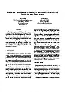
Abstract— In this paper, we present a real-time algorithm for local simultaneous localization and mapping (SLAM) with detection and tracking of moving objects (DATMO) in dynamic outdoor environments from a moving vehicle equipped with a laser scanner. To correct vehicle location from odometry we introduce a new fast implementation of incremental scan matching method that can work reliably in dynamic outdoor environments. After a good vehicle location is estimated, the surrounding map is updated incrementally and moving objects are detected without a priori knowledge of the targets. Detected moving objects are finally tracked by a Multiple Hypothesis Tracker (MHT) coupled with an adaptive IMM (Interacting Multiple Models) Filter. The experimental results on datasets collected from different scenarios such as: urban streets, country roads and highways demonstrate the efficiency of the proposed algorithm on a Daimler Mercedes demonstrator in the framework of the European Project PReVENT-ProFusion2. Fig. 1.

The Daimler Mercedes demonstrator car.

I. INTRODUCTION Perceiving or understanding the environment surrounding of a vehicle is a very important step in driving assistant systems or autonomous vehicles. The task involves both simultaneous localization and mapping (SLAM) and detection and tracking of moving objects (DATMO). While SLAM provides the vehicle with a map of static parts of the environment as well as its location in the map, DATMO allows the vehicle being aware of dynamic entities around, tracking them and predicting their future behaviors. It is believed that if we are able to accomplish both SLAM and DATMO in real time, we can detect every critical situations to warn the driver in advance and this will certainly improve driving safety and can prevent traffic accidents. Recently, there have been considerable research efforts focusing on these problems [6][11]. However, for highly dynamic outdoor environments like crowded urban streets, there still remains many open questions. These include, how to represent the vehicle environment, how to obtain a precise location of the vehicle in presence of dynamic entities, and how to differentiate moving objects and stationary objects as well as how to track moving objects over time. In this context, we design and develop a generic architecture to solve SLAM and DATMO in dynamic outdoor environments. This architecture (Fig. 2) is divided into two main parts: the first part where the vehicle environment is mapped, fusion between different sensors is performed and moving objects are detected; and the second part where previously detected moving objects are verified and tracked. This architecture is currently used in the framework of the

European project PReVENT-ProFusion1 . The goal of this project is to design and develop generic architectures to perform perception tasks (ie, mapping of the environment, localization of the vehicle in the map, and detection and tracking of moving objects). In this context, our architecture has been integrated and tested on two demonstrators: a Daimler-Mercedes demonstrator and a Volvo truck demonstrator. In previous paper [10], a description of the first level is reported. In this paper, we detail the description of the sensor data fusion part of the first level and the second level and show some results on the Daimler-Mercedes demonstrator moving at high speed. The rest of the paper is organized as follows. In the next section, we present the Daimler Mercedes demonstrator. A brief overview of our architecture is given in section III. Description of first level of architecture is summarized and Sensor Data Fusion is described in Section IV. Second level is detailed in section V. Experimental results are given in Section VI and finally in Section VII conclusions and future works are discussed. II. THE DAIMLER MERCEDES DEMONSTRATOR The DaimlerChrysler demonstrator car is equipped with a camera, two short range radar sensors and a laser scanner (Fig. 1). The radar sensor is with a maximum range of 30m and a field of view of 80◦ . The maximum range of laser sensor is 80m with a field of view of 160◦ and a horizontal 1 www.prevent-ip.org/profusion

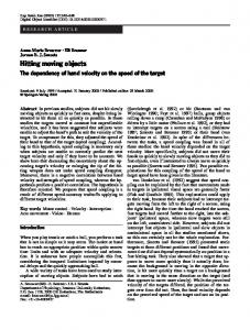
Fig. 3.

Moving object detection example. See text for more details.

A. Environment Mapping & Localization

Fig. 2.

Architecture of the perception system

resolution of 1◦ . In addition, vehicle odometry information such as velocity and yaw rate are provided by the vehicle sensors. The measurement cycle of the sensor system is 40ms. Images from camera are for visualization purpose. III. GENERAL ARCHITECTURE We design and develop a generic architecture (Fig. 2) to solve SLAM and DATMO in dynamic outdoor environments. In the first part of the architecture, to model the environment surrounding the vehicle, we use the Occupancy Grid framework developed by Elfes [4]. Compared with featurebased approaches, grid maps can represent any environment and are specially suitable for noisy sensors in outdoor environments where features are hard to define and extract. In general, in order to perform mapping or modelling the environment from a moving vehicle, a precise vehicle localization is essential. To correct vehicle locations from odometry, we introduce a new fast laser-based incremental localization method that can work reliably in dynamic environments. When good vehicle locations are estimated, by integrating laser measurements we are able to build a consistent grid map surrounding of the vehicle. Finally by comparing new measurements with the previously constructed local vehicle map, dynamic objects then can be detected. Finally, sensor data coming from different sensors are fused. In the second part, detected moving objects in the vehicle environment are tracked. Since some objects may be occluded or some are false alarms, multi objects tracking helps to identify occluded objects, recognize false alarms and reduce mis-detections. IV. FIRST LEVEL In this section, we first summarized the description of the first level of our architecture: Environment Mapping & Localization, Moving Objects Detection. More details on the two first parts could be found in [10]. In the last subsection, we describe the fusion between objects detected by laser and radar data.

To map the environment and localize in the environment, we propose an incremental mapping approach based on a fast laser scan matching algorithm in order to build a consistent local vehicle map. The map is updated incrementally when new data measurements arrive along with good estimates of vehicle locations obtained from the scan matching algorithm. The advantages of our incremental approach are that the computation can be carried out very quickly and the whole process is able to run online. 1) Environment mapping using Occupancy Grid Map: Using occupancy grid representation, the vehicle environment is divided into a two-dimensional lattice M of rectangular cells and each cell is associated with a measure taking a real value in [0, 1] indicating the probability that the cell is occupied by an obstacle. A high value of occupancy grid indicates the cell is occupied and a low value means the cell is free. Suppose that occupancy states of individual grid cells are independent, the objective of a mapping algorithm is to estimate the posterior probability of occupancy P(m | x1:t , z1:t ) for each cell of grid m, given observations z1:t = {z1 , ..., zt } from time 1 to time t at corresponding known poses x1:t = {x1 , ..., xt }.from time 1 to time t. 2) Localization of the vehicle in the Occupancy Grid Map: In order to build a consistent map of the environment, a good vehicle localization is required. Because of the inherent error, using only odometry often results in an unsatisfying map. To solve this problem, we used a particle filter. We predict different possible positions of the vehicle (ie, one position of the vehicle corresponds to one particle) using the motion model and compute the probability of each position (ie, the probability of each particle) using the laser data and a sensor model. B. Moving Objects Detection After a consistent local grid map of the vehicle is constructed, moving objects can be detected when new laser measurements arrive by comparing with the previously constructed grid map. The principal idea is based on the inconsistencies between observed free space and occupied space in the local map. If an object is detected on a location previously seen as free space, then it is a moving object. If an object is observed on a location previously occupied then it probably is static. If an object appears in a previously not observed location, then it can be static or dynamic and we set the unknown status for the object in this case.

Fig. 4. Moving object detected from laser data is confirmed by radar data.

Fig. 3 illustrates the described steps in detecting moving objects. The leftmost image depicts the situation where the vehicle is moving along a street seeing a car moving ahead and a motorbike moving in the opposite direction. The middle image shows the local static map and the vehicle location with the current laser scan drawn in red. Measurements which fall into free region in the static map are detected as dynamic and are displayed in the rightmost image. After the clustering step, two moving objects are identified (in green boxes) and correctly corresponds to the car and the motorbike. C. Fusion with radars After moving objects are identified from laser data, we confirm the object detection results by fusing with radar data and provide the detected objects with their velocities. For each moving object detected from laser data as described in the previous section, a rectangular bounding box is calculated and the radar measurements which lie within the box region are then assigned to corresponding object. The velocity of the detected moving object is estimated as the average of these corresponding radar measurements. Figure 4 shows an example of how the fusion process takes place. Moving objects detected by the Laserscanner are displayed in red with green bounding boxes. The targets detected by two radar sensors are represented as small circles in different colors along with corresponding velocities. We can see in the radar field of view, that two objects detected by the Laserscanner are also seen by two radars so that they are confirmed and their velocities are estimated. Radar measurements that do not correspond to any dynamic object or fall into another region of the grid are not considered. V. SECOND LEVEL In general, the multi objects tracking problem is complex: it includes the definition of tracking methods, but also association methods and maintenance of the list of objects currently present in the environment [2][9]. Regarding tracking techniques, Bayesian filters [1] are generally used. These filters require the definition of a specific motion model of tracked objects to predict their positions in the environment. Using this prediction and some observations, in a second stage, an estimation of the position of each object present in the environment is computed.

In this section, we describe the four different parts of our architecture (figure 2) to solve the different parts of multiobjects tracking: • The first one is the gating. In this part, taking as input predictions from previous computed tracks, we compute the set of new detected objects which can be associated to each track. • In a second part, using the result of the gating, we perform objects to tracks association and generate association hypothesis, each track corresponding to a previously known moving object. Output is composed of the computed set of association hypothesis. • In the third part called tracks management, tracks are confirmed, deleted or created according to the association results and a pruned set of association hypothesis is output. • In the last part corresponding to the filtering step, estimates are computed for ’surviving’ tracks and predictions are performed to be used the next step of the algorithm. In this part, we use an adaptive method based on Interacting Multiple Models (IMM). More details about these different parts are outlined next. A. Gating In this part, taking as input predictions from previous computed tracks and newly detected objects, a gating is performed. It consists in, according to an arbitrary distance function, determine the detected objects which can be associated with tracks. Also during this stage, clustering is performed in order to reduce the number of association hypothesis. It consists in making clusters of tracks which share at least one detected object. In the next stage, association can be performed independently for each cluster decomposing a large problem in smaller problems which induce generation of less hypothesis.

Fig. 5.

Example of association problem

If we take as an example the situation depict by the Fig. 5, in this stage one set is computed as T1 and T2 share object O2 . Also according to gates, objects O1 and O2 can be assigned to T1 and objects O2 and O3 to T3 . B. Association In this part, taking as input clusters of tracks and detected objects validated by the gating stage, association hypothesis are evaluated. By considering likelihood of objects with tracks, new track apparition probability and non-detection probability, an association matrix is formed. Let be L(oi ,t j ) the function giving the likelihood of object i with track j, PNT the new track apparition probability and

PND the non detection probability. Taking as an example the situation in the Figure 5, the association matrix is written:   L(o1 ,t1 ) −∞ PNT  L(o2 ,t1 ) L(o2 ,t2 ) PNT     −∞ L(o3 ,t2 ) PNT  PND PND −∞ Thus a possible association hypothesis corresponds to a valid assignation in the matrix of detected objects with tracks i.e one unique element in each row and each column is chosen to compose the assignation. In order to reduce the number of hypothesis, only the m-best association hypothesis are considered. The m-best assignment in the association matrix are computed using the Murty method [7] which computes the m-Best assignations in the matrix and by this way we obtain the m-Best Hypothesis. C. Track management In this third stage, using the m-Best Hypothesis resulting of the association stage, the set of tracks, is maintained i.e tracks are confirmed, deleted or created. New tracks are created if a new track creation hypothesis appears in the m-best hypothesis. A new created track is confirmed if it is updated by detected objects after a fixed number of algorithm steps (three in our implementation). Thus spurious measurements which can be detected as objects in the first step of our method are never confirmed. If a non-detection hypothesis appears and so to deal with non-detection cases (which can appear for instance when an object is occulted by an other one, tracks without associated detected objects are updated according to their last associated objects and next filtering stage becomes a simple prediction. But if a track is not updated by a detected object for a given number of steps, it is deleted. D. Adaptive Filtering using Interacting Multiple Models In this filtering stage, according to previously computed predictions, estimations are performed for each association of all hypothesis and new predictions are computed for the gating stage. Regarding filtering techniques, there exists several kinds of filters, the most classical is the well known Kalman filter. But in all kinds of filters, the motion model is the main part of the prediction step. To deal with these motion uncertainties, Interacting Multiple Models (IMM) [8] have been successfully applied in several applications [3]. The IMM approach overcomes the difficulty due to motion uncertainty by using more than one motion model. The principle is to assume a set of motion models as possible candidates of the true displacement model of the object at one time. To do so, a bank of elemental filters is ran at each time, each corresponding to a specific motion model, and the final state estimation is obtained by merging the results of all elemental filters according to the distribution probability over the set of motion models (in the next part we note µ this probability). By this way different motion models are taken into account during filtering process.

Fig. 6.

Principle of our adaptive filtering program

As the quality of gating relies directly on the quality of filtering and especially the prediction step, we have chosen Interacting Multiple Models (IMM) [8] to deal with motion uncertainties in this filtering part. Besides, we developed an efficient method in which critical parameter of the IMM is on-line adapted according to the most probable trajectories formed by tracks. Thus as Fig. 6 shows our filtering stage is composed of three parts : an IMM filtering part, a part in which most probable trajectories are computed and a last part in which we adapt the IMM filter. These three parts are described in the next paragraphs.

Fig. 7.

The sixteen chosen motion models in the vehicle’s frame

1) Definition of our IMM: Nevertheless, to apply IMM on real applications a number of critical parameters have to be defined, for instance the set of motion models and the transition probability matrix(TPM). To cope with this design step which can no match the reality, we propose an efficient method in which the TPM is on-line adapted. In our specific application, different objects such as cars or motorcycles can move in any directions and can often change their motions. Thus in our aim we choose various IMM’s motion models to cover the set of possible directions and velocities. As each filter corresponds to a specific motion model, we have to define each motion model. So, assuming we have different possible velocities defined according to the vehicle velocity and eight directions in the set of possible directions an object can follow, we obtain sixteen motion models (Fig. 7). Hence, according to the definition of these sixteen motion models, our IMM is composed of sixteen kalman filters. The TPM is initially chosen to be uniform. 2) Computation of the most probable trajectories: Once estimates are performed for all hypothesis, the most probable

trajectory is computed for each track. This step permits to give users more readability on what is happening during tracking process and also permits us to adapt on-line the IMM parameter according to these trajectories. 3) Adaptation of the IMM: To adapt the TPM in our specific situation i.e tracking detected objects, most probable trajectories are considered. Taking as input the set of trajectories computed during filtering process, we will adapt online the TPM of the IMM filter in order to obtain a better transition between motion models close to the real behavior of tracked objects. The principle is the following. For a given number N of trajectories we build sequences of associated motion models probabilities. And then, using these motion models probabilities, the TPM is adapted and reused in the IMM filters for the next estimations. In more details, algorithm 1, given in pseudo-code, is the algorithm defined to compute one adaptation of the TPM. Algorithm 1 Adaptive IMM Algorithm 1: Adaptation of TPM(T0 , ..., TN ) 2: n ← 0 3: repeat 4: Sn ← [ ] 5: /* Store µk ,...µk′ from Tn the most probable nth trajectory */ 6: for all Ob ject pose xk in Tn do 7: {µk } ← Tn (k) 8: Sn ← Sn ∪ [µk ] 9: end for 10: /* Compute the most probable model sequence MPS */ 11: MPS ← Viterby(Sn ) 12: /* Quantification of model transitions */ 13: for all Couple ( MPSk , MPSk+1 ) in MPS do 14: i ← MPSk 15: j ← MPSk+1 16: Fi j = Fi j + 1 17: end for 18: n ← n+1 19: until n = N 20: /* Update of TPM in IMM */ 21: T PM ← Normalization(F) 22: Return TPM in IMM An adaptation of the TPM is done after a given number N of trajectories obtained from tracks, to update TPM using a window on trajectories (cf. loop line 3-19 of algorithm 1). Moreover trajectories are processed one by one in three steps: 1- Models’ probabilities are collected by travel through the computed most probable sequence 2- Most probable models’ sequence is computed 3- Most probable models’ transitions are quantified Collection of models’ probabilities : : For each part of a given most probable trajectory computed in last stages of the

filtering process, we collect the distribution over models(lines 7). Thus a model probabilities’ sequence Sn obtained in such a way and is stored to be processed (line 8). Computation of the most probable model sequence : : In a next step, the most probable models’ sequence of Sn is computed (line 11). More precisely, considering the actual TPM and a set Sn = µ0 ...µK of model probabilities through time 0 to K, we aim to obtain the most probable models’ sequence knowing the estimates computed by the IMM: Max P(µ0 µ1 ...µk | x0 x1 ... xK )

(1)

We just need to obtain the maximum of the distribution P(µ1 µ2 ...µK | x0 x1 ... xK ), thus the inference is made using the Viterbi Data Algorithm [5]. As complexity of this algorithm is in O(KM 2 ), we efficiently obtain the most probable models’ sequence. Quantification of most probable model transitions : : Using this most probable models’ sequence, the number of transitions from one model to an other is quantified (lines 13 to 17). To do so a frequencies matrix is considered. This matrix models the number of transitions which have occurred from one model to an other. We note F this matrix and so Fi j gives the number of transitions which has occurred from model i to j. Using the most probable models’ sequence corresponding to a specific trajectory and computed by the Viterbi algorithm, the update of F is directly obtained by counting transitions in this sequence. Furthermore, F is kept in memory to be used in next adaptation and before the first update all its elements are set to 1. Finally, when N trajectories have been treated, the new TPM is obtained by normalization of the frequencies matrix F. Thus the TPM is re-estimated using all model sequences S1 ...SN and is reused in the IMM for next executions (lines 21 and 22). In practice, before the first run, the TPM is chosen uniform (according to F initialization) as we do not want to introduce a priori data. VI. EXPERIMENTAL RESULTS The detection and tracking results are shown in Fig. 8. The images in the first row represent online maps and objects moving in the vicinity of the vehicle are detected and tracked. The current vehicle location is represented by blue box along with its trajectories after correction from the odometry. The red points are current laser measurements that are identified as belonging to dynamic objects. Green boxes indicate detected and tracked moving objects with corresponding tracks displayed in different colors. Information on velocities is displayed next to detected objects if available. The second row are images for visual references to corresponding situations. In Fig. 8, the leftmost column depicts a scenario where the demonstrator car is moving at a very high speed of about 100 kph while a car moving in the same direction in front of it is detected and tracked. On the rightmost is a situation where the demonstrator car is moving at 50 kph on a country road. A car moving ahead and two other cars in the opposite direction are all recognized. Note that the two cars on the

Fig. 8.

Experimental results show that our algorithm can successfully perform both SLAM and DATMO in real time for different environments

left lane are only observed during a very short period of time but both are detected and tracked successfully. The third situation in the middle, the demonstrator is moving quite slowly at about 20 kph in a crowded city street. Our system is able to detect and track both the other vehicles and the motorbike surrounding. In all three cases, precise trajectories of the demonstrator are achieved and local maps around the vehicle are constructed consistently. In our implementation, the computational time required to perform both SLAM and DATMO for each scan is about 20 − 30 ms on a 1.86GHz, 1Gb RAM laptop running Linux. This confirms that our algorithm is absolutely able to run synchronously data cycle in real time. More results and videos can be found at http: //emotion.inrialpes.fr/∼tdvu/videos/. VII. CONCLUSIONS AND FUTURE WORKS We have presented an approach to accomplish online mapping and moving object tracking simultaneously. Experimental results have shown that our system can successfully perform a real time mapping and moving object tracking from a vehicle at high speeds in different dynamic outdoor scenarios. This is done based on a fast scan matching algorithm that allows estimating precise vehicle locations and building a consistent map surrounding of the vehicle. After a consistent local vehicle map is built, moving objects are detected and are tracked using an adaptive Interacting Multiple Models filter coupled with an Multiple Hypothesis tracker.

VIII. ACKNOWLEDGMENTS The work is supported by the European project PReVENTProFusion, and partially by the Délégation Générale pour L’Armement (DGA). R EFERENCES [1] S. Arulampalam, S Maskell, N Gordon, and T Clapp. A tutorial on particle filter for online nonlinear/non-gaussian bayesian tracking. IEEE Transactions on Signal Processing, 50(2), 2002. [2] Y. Bar-Shalom and T.E. Fortman. Tracking and Data Association. Academic Press, 1988. [3] S. Blackman and R. Popoli. Design and Analysis of Modern Tracking Systems. Artech House, 2000. [4] A. Elfes. Occupancy grids: a probabilistic framework for robot percpetion and navigation. PhD thesis, Carnegie Mellon University, 1989. [5] G. David Forney. The viterbi algorithm. Proceedings of The IEEE, 61(3):268–278, 1973. [6] D. Hähnel, D. Schulz, and W. Burgard. Mobile robot mapping in populated environments. Advanced Robotics, 17(7):579–598, 2003. [7] K. G. Murty. An algorithm for ranking all the assignments in order of increasing costs. Operations Research, 16:682–687, 1968. [8] X. Rong Li and Vesselin P.Jilkov. A survey of maneuvering target tracking-part v: Multiple-model methods. IEEE Transactions on Aerospace and Electronic Systems, 2003. [9] S. Thrun, W. Burgard, and D. Fox. Probabilistic Robotics (Intelligent Robotics and Autonomous Agents). The MIT Press, September 2005. [10] TD. Vu, O. Aycard, and N. Appenrodt. Online localization and mapping with moving objects tracking in dynamic outdoor environments. In IEEE International Conference on Intelligent Vehicles, 2007. [pdf]. [11] C.-C. Wang. Simultaneous Localization, Mapping and Moving Object Tracking. PhD thesis, Robotics Institute, Carnegie Mellon University, Pittsburgh, PA, April 2004.