w in Li . Consider a Stick representation of PG where the elements of V correspond to vertical sticks. Restricting the linear extensions L1 = L← , L2 = L→ , and L3 = L↑ (cf. the proof of Proposition 6) obtained from a Stick representation of PG to the elements of V yields linear orders satisfying the property above. Thus G is outerplanar. For the backward direction let G be an outerplanar graph. In [3] it is shown that the class of hook contact graphs (each intersection of hooks is also an endpoint of a hook) is exactly the class of outerplanar graphs. Given a hook contact representation of G we construct a Stick representation of PG . To this end we consider each hook as two sticks, a vertical one for the vertices and a horizontal one as a placeholder for the edges. For each contact of the
12
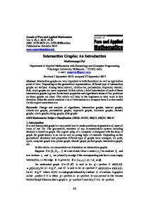
horizontal part of a hook v we place an additional horizontal stick slightly below the center of v. The k-th contact of a hook with the horizontal part is realized by the k-th highest edge that is added in the placeholder as shown in Figure 8.
Figure 8: A hook contact representation of G transformed into a Stick representation of PG . We continue by providing some characterizations of outerplanar graphs according to GIG representations of vertex-edge incidence posets. A weak semibar-visibility representation of a graph is a drawing that represents the vertices as vertical segments with lower end at the horizontal line y = 0, and the edges as horizontal segments touching the two vertical segments that represent incident vertices. Lemma 2 ([8]) A graph G is outerplanar if and only if G has a weak semibar-visibility representation. The construction used in the previous proposition directly produces a weak semibarvisibility representation of an outerplanar graph. Just extend all vertical segments upwards until they hit a common horizontal line ` and reflect the plane at `, now ` can play the role of the x-axis for the weak semibar-visibility representation. Proposition 11 A graph G is outerplanar if and only if the graph PG has a SegRay representation where the vertices of G are represented as rays. Proof. Cutting the rays of a SegRay representation with rays pointing downwards somewhere below all horizontal segments leads to a weak semibar-visibility representation of G and vice versa. Thus, Lemma 2 gives the result. Proposition 12 A graph G is outerplanar if and only if the graph PG has a hook representation. Proof. If G is outerplanar then PG has a hook representation by Proposition 10. On the other hand, assume that PG has a hook representation for a graph G. According to Proposition 5 we construct a SegRay representation with vertices as rays and edges as segments. This representation shows that G is outerplanar by Proposition 11. Proposition 13 If G is outerplanar, then the graph PG has a SegRay representation where the vertices of G are represented as segments.
13
Proof. Consider a hook representation R0 of PG . According to the proof Proposition 5 we can transform PG into a SegRay representation with a free choice of the colorclass that is represented by rays. Choosing the subdivision vertices as rays leads to the required representation.
Figure 9: A SegRay representation of PK2,3 . In contrast to Proposition 11, the backward direction of Proposition 13 does not hold: Figure 9 shows a SegRay representation of PK2,3 with vertices being represented as horizontal segments, but K2,3 is not outerplanar. Together with Proposition 11 this also shows that the class of SegRay graphs is not symmetric in its color classes. In the following we construct a UGIG representation of PG for an outerplanar graph G. Proposition 14 If G is outerplanar then PG is a UGIG. Proof. We construct a UGIG representation of PG for a maximal outerplanar graph G = (V, E) with outer-face cycle v0 , . . . , vn . The vertices of V are drawn as vertical segments. Starting from v0 we iteratively draw the vertices of breadth-first-search layers (BFS-layers). Each BFS-layer has a natural order inherited from the order on the outer-face, i.e., the increasing order of indices. When the i-th layer Li has been drawn the following invariants hold: 1. Segments for all vertices and edges of G[L0 , . . . , Li−1 ], all vertices of Li , and all edges connecting vertices of Li−1 to vertices of Li have been placed. 2. The upper endpoints of the segments representing vertices in Li lie on a strict monotonically decreasing curve Ci . Their order on Ci agrees with the order of the corresponding vertices in Li . Their x-coordinates differ by at most one. 3. No segment intersects the region above Ci . We start the construction with the vertical segment corresponding to v0 . The curve C0 is chosen as a line with negative slope that intersects the upper endpoint of v0 . We start the (i + 1)-th step by adding segments for the edges within vertices of layer Li . Afterwards we add the segments for edges between vertices in layer Li and Li+1 and the segments for the vertices of layer Li+1 . The construction is indicated in Figure 10. First we draw unit segments for the edges within layer Li . Since the graph is outerplanar such edges only occur between consecutive vertices of the layer. For a vertex vk of Li which is not the first vertex of Li we define a horizontal ray rk whose start is on the segment of
14
Ci
Ci
Ci
Ci+1
rl rm vk vl a)
vm
b)
c)
Figure 10: One step in the construction of a UGIG representation of PG : a)The situation before the step. b) The edges between layer Li and Li+1 and within layer Li are added. c) The vertices of layer Li+1 are added. the predecessor of vk on this layer such that the only additional intersection of rk is with the segment of vk . The initial unit segment of ray rk can be used for the edge between vk and its predecessor. All segments that will represent edges between layer Li and Li+1 are placed as horizontal segments that intersect the segment of the incident vertex vk ∈ Li above the ray rk . We draw these edge-segments such that the endpoints lie on a monotonically decreasing curve C and the order of these endpoints on C corresponds to the order of their incident vertices in Li+1 . Now the right endpoints of the edges between the two layers lie on the monotone curve C and no segment intersects the region above this curve. Due to properties of the BFS for outerplanar graphs, each vertex of layer Li+1 is incident to one or two edges whose segments end on C and if there are two then they are consecutive on C. We place the unit segments of vertices of Li+1 , such that their lower endpoint is on the lower segment of an incident edge with the x-coordinate such that they realize the required intersections. With this construction the invariants are satisfied. There are graphs G where PG is a UGIG and G is not outerplanar, for example G = K2,3 as shown in Figure 11. On the other hand there exist planar graphs G, such that PG is not a UGIG as the following proposition shows. Proposition 15 PK4 is not a UGIG. Proof. Suppose to the contrary that PK4 has a UGIG representation with vertices as vertical segments. By contracting vertical segments to points one can obtain a planar embedding of K4 from such a representation. As K4 is not outerplanar, there is a vertex v that is not incident to the outer face in this embedding. For the initial UGIG representation this means that v is represented by a vertical segment which is enclosed by segments representing vertices and edges of K4 − {v}. Notice that these segments represent a 6-cycle of PK4 . However, the largest vertical distance between any pair of horizontal segments in this cycle
15
is less than 1. Thus, there is not enough space for the vertical segment of v, contradiction.
Figure 11: A UGIG representation of PK2,3 .
5 Separating examples In this section we will give examples of graphs that separate the graph classes in Figure 1. For this purpose we will show that the classes we have observed to be at most 4-dimensional indeed contain 4-dimensional graphs. This is done in Subsection 5.1 using standard examples and vertex-face incidence posets of outerplanar graphs. The remaining graph classes will be separated using explicit constructions in Subsection 5.2 and Subsection 5.3. Using the observations of Section 4 about vertex-edge incidence posets we can immediately separate the following graph classes. StabGIG 6⊂ BipHook
StabGIG 6⊂ 3-DORG
SegRay 6⊂ 4-DORG
Stick 6⊂ 2-DORG.
In [25] it is shown that the graph C14 (cycle on 14 vertices) is not a 4-DORG, and in particular is not a 3- or 2-DORG. In other words, PC7 is not a 4-DORG. Since C7 is outerplanar, by the propositions of the previous section we know that PC7 is a SegRay, a StabGIG and a Stick graph. This shows the three seperations involving DORGs. For the first one let G be a planar graph that is not outerplanar. Then PG is a StabGIG (Proposition 9) but not a BipHook graph (Proposition 12).
5.1 4-Dimensional Graphs First of all, some graph classes are already separated by their maximal dimension. The standard example Sn of an n-dimensional poset, cf. [30], is the poset on n minimal elements a1 , . . . , an and n maximal elements b1 , . . . , bn , such that ai < bj in Sn if and only if i 6= j. To separate most of the 4-dimensional classes from the 3-dimensional ones, the standard example S4 is sufficient. As shown in Figure 12 it has as a stabbable 4-DORG representation.
16
11 00 00 11 00 11
11 00 00 11 00 11
11 00 00 11 00 11
111 000 000 111 000 111
111 000 000 111 000 111
11 00 00 11 00 11
111 000 000 111 000 111
11 00 00 11 00 11
Figure 12: The poset S4 and a stabbable 4-DORG representation of it. From this it follows that: StabGIG 6⊂ BipHook
StabGIG 6⊂ 3-DORG
4-DORG 6⊂ 3-DORG
StabGIG 6⊂ 3-dim GIG
Since the interval dimension of Sn is n we get the following relations from Proposition 7. StabGIG 6⊂ SegRay
4-DORG 6⊂ SegRay
We will now show that the vertex-face incidence poset of an outerplanar graph has a SegRay representation. In [15] it has been shown that there are outerplanar maps with a vertex-face incidence poset of dimension 4. Together with Proposition 16 below this shows that there are SegRay graphs of dimension 4. We obtain SegRay 6⊂ 3-dim GIG. Proposition 16 If G is an outerplanar map then the vertex-face incidence poset of G is a SegRay graph. Let G be a graph with a fixed outerplanar embedding. First we argue that we may assume that G is 2-connected. If G is not connected then we can add a single edge between two components without changing the vertex-face poset. Now consider adding an edge between two neighbours of a cut vertex on the outer face cycle, i.e., two vertices of distance 2 on this cycle. This adds a new face to the vertex-face-poset, but keeps the old vertex-face-poset as an induced subposet. Therefore, we may assume that G is 2-connected. v2
v1
f v1
v2
f
v2
v1
f
Figure 13: Illustration for the induction step in Proposition 16 By induction on the number of bounded faces we show that G has a SegRay representation in which the cyclic order of the vertices on the outer face agrees with the left-right order (cyclically) of rays representing these vertices. If G has one bounded face then the claim is
17
straight-forward. If G has more bounded faces then consider the dual graph of G without the outer face, which is a tree. Let f be a face that corresponds to a leaf of that tree. Define G0 to be the plane graph obtained by removing f and incident degree-2 vertices from G. Then exactly two vertices v1 , v2 of f are still in G0 , and they are adjacent via an edge at the outer face of G0 . Note that G0 is 2-connected. Applying induction on G0 we obtain a SegRay representation in which the two rays representing v1 and v2 are either consecutive, or left- and rightmost ray. In the first case we insert rays for the removed vertices between v1 and v2 with endpoints being below all other horizontal segments. Then a segment representing f can easily be added to obtain a SegRay representation with the required properties of G, see the middle of Figure 13. If the rays of v1 and v2 are the left- and rightmost ones, then observe that the endpoints of both rays can be extended upwards to be above all other endpoints. We can insert the new rays to the left of all the other rays and the segment for f as indicated in Figure 13 on the right. This concludes the proof. Propositions 16 and 7 also give the following interesting result about vertex-face incidence posets of outerplanar maps which complements the fact that they can have dimension 4 [15]. Corollary 2 The interval dimension of a vertex-face incidence poset of an outerplanar map is bounded by 3. We have separated all the graph classes which involve dimension except for the two classes of 3-dimensional GIGs and stabbable GIGs. As indicated in Figure 1 it remains open whether 3-dim GIG is a subclass of StabGIG or not. More comments on this can be found at the end of Subsection 5.3.
5.2 Constructions In this subsection we give explicit constructions for the remaining separations of classes not involving StabGIG. In the introduction we mentioned that every 2-dimensional order of height 2, i.e., every bipartite permutation graph, is a GIG. We show now that this does not hold for 3-dimensional orders of height 2. Proposition 17 There is a 3-dimensional bipartite graph that is not a GIG. Proof. The left drawing in Figure 14 defines a poset P by ordering the homothetic triangles by inclusion. Some of the triangles are so small that we refer to them as points from now on. Each inclusion in P is witnessed by a point and a triangle, and hence P has height 2. To see that it is 3-dimensional we use the drawing and the three directions depicted in Figure 14. By applying the same method as we did for Proposition 6 we obtain three linear extensions forming a realizer of P . We claim that P is not a pseudosegment intersection graph1 , and hence not a GIG. Suppose to the contrary that it has a pseudosegment representation. The six green triangles together with the three green and the three blue points form a cycle of length 12 in G. 1
The intersection graph of curves where each pair of curves intersects in at most one point.
18
1111 0000 1111 0000 1111 0000 1111 0000 1111 0000 1111 0000 1111 0000
1111 0000 1111 0000 1111 0000 1111 0000
000 111 000 111 000 111 000 111 000 111 000 111 000 111 000 111
Figure 14: The drawing on the left defines an inclusion order of homothetic triangles. This height-2 order does not have a pseudosegment representation. Hence, the union of the corresponding pseudosegments in the representation contains a closed curve in R2 . Without loss of generality assume that the pseudosegment representing the yellow point lies inside this closed curve (we may change the outer face using a stereographic projection). The pseudosegments of the three large blue triangles intersect the yellow pseudosegment and one blue pseudosegment (corresponding to a blue point) each. The yellow and the blue pseudosegments divide the interior of the closed curve into three regions. We show that each of these regions contains one of the pseudosegments representing black points. Each purple pseudosegment intersects the cycle in a point that is incident to one of the three bounded regions. Now, each black pseudosegment intersects a purple one. If such an intersection lies in the unbounded region, then the whole black pseudosegment is contained in this region. This is not possible as for each of the black pseudosegments there is a blue pseudosegment representing a small blue triangle that connects it to the enclosed yellow pseudosegment without intersecting the cycle. Thus, the three intersections of purple and black pseudosegments have to occur in the bounded regions, and in each of them one. It follows that each of the three bounded regions contains one black pseudosegment. Now, the red pseudosegment intersects each of the three black pseudosegments. Since they lie in three different regions whose boundary it may only traverse through the yellow pseudosegment, it has to intersect the yellow pseudosegment twice. This contradicts the existence of a pseudosegment representation. In the following we give constructions to show that Stick 6⊂ UGIG
UGIG 6⊂ Stick
BipHook 6⊂ 3-DORG
BipHook 6⊂ Stick
Proposition 18 The Stick graph shown in Figure 15 is not a UGIG.
19
Figure 15: A stick representation of a graph that is not a UGIG. Proof. Let G be the graph represented in Figure 15. Let v and h be the two adjacent vertices of G that are drawn as black sticks in the figure. There are five pairs of intersecting blue vertical and red horizontal segments v1 , h1 , . . . , v5 , h5 . Each vi intersects h and each hi intersects v. Four of the pairs vi , hi form a 4-cycle with a pair of green segments qi , ri . Suppose that G has a UGIG representation. We claim that in any such representation the intersection points pi of vi and hi form a chain in