Aug 5, 2017 - Subhabrata Paul â¡. August 8, 2017. Abstract ... CG] 5 Aug 2017 .... Figure 5: Conversion of a straight line edge into a Manhattan path those grid ...
Grid obstacle representation of graphs Arijit Bishnu
∗
Arijit Ghosh
∗
Rogers Mathew
†
Subhabrata Paul
‡
August 8, 2017
arXiv:1708.01765v1 [cs.CG] 5 Aug 2017
Abstract The grid obstacle representation of a graph G = (V, E) is an injective function f : V → Z2 and a set of point obstacles O on the grid points of Z2 (where V has not been mapped) such that uv is an edge in G if and only if there exists a Manhattan path between f (u) and f (v) in Z2 avoiding the obstacles of O. The grid obstacle number of a graph is the smallest number of obstacles needed for the grid obstacle representation of G. This work shows that planar graphs admit such a representation while there exists some non-planar graphs that do not admit such a representation. Moreover, we show that every graph admits grid obstacle representation in Z3 . We also show NP-hardness result for the point set embeddability of an `1 -obstacle representation. Keywords. Geometric graph, grid obstacle representation, obstacle number
1
Introduction
In 2010, Alpert et al. [AKL10] introduced the concept of obstacle representation of a graph which is closely related to visibility graphs [Gho07, GG13, GO97]. Their attempt was to represent every graph G = (V, E), |V | = n, |E| = m, in the Euclidean plane with a point set P = V and a set O of polygonal obstacles such that for every edge pq ∈ E, p and q are visible in the Euclidean plane and every non-edge (a non-edge is a pair of vertices p, q ∈ V with pq 6∈ E) is blocked by some obstacle o ∈ O. The smallest number of obstacles needed to represent a graph G is called the obstacle number of G and is denoted by obs(G). Clearly, obs(G) ≤ n(n − 1)/2. Starting with the work of Alpert et al. [AKL10], there have been several studies [BCV15, DM15, FSS11, JS11, JS14, MPP12, MPS10, PS11, Sar11] on existential and optimization related questions on obstacle number. In [AKL10], Alpert et al. identified some √ families of graphs having obstacle number 1 and constructed graphs with obstacle number Ω( log n). Dujmovic et al. [DM15] proved a lower bound of Ω(n/(log log n)2 ) on obstacle number. Balko et al. [BCV15] showed that the obstacle number for general graphs is O(n log n) and for graphs with bounded chromatic number it is O(n). Pach et al. [PS11] showed the existence of graphs with arbitrarily large obstacle number using extremal graph theory.
1.1
The Definition
The essence of obstacle representation of a graph is about blocking the visibility in the Euclidean plane among pairs of points whose corresponding vertices do not have an edge. The idea of “blocking visibility” [DPT09, Mat09] between pairs of points in the Euclidean plane with a minimum set of point obstacles or blockers has resonance with the obstacle representation – consider the obstacle representation of a graph with a finite number of vertices but no edges. ∗
Indian Statistical Institute, Kolkata, India Indian Institute of Technology - Kharagpur, India ‡ Indian Institute of Information Technology Guwahati, India †
1
v2 v1
v2
v1
v3
v3
v4
v4
Figure 1: Grid obstacle representation of a graph; the `1 -obstacle representation is on the right for the graph on the left side.
In the Euclidean plane, the shortest path and straight line visibility are essentially the same. To generalize the definition of obstacle representation to other metric spaces, we replace visibility blocking in the Euclidean plane by shortest path blocking in a metric space. An obstacle representation of a graph G = (V, E) in a metric space (M, δ) consists of a mapping from V to P ⊆ M and a set of point obstacles to be placed on points of M. We would say that in a metric space (M, δ), two points p1 , p2 ∈ P ⊆ M are visible if at least one shortest path between p1 and p2 is neither blocked by any obstacle, nor by any point of P . Do observe that the shortest paths in M depend on the metric δ, and need not be unique. Definition 1 (Obstacle representation problem). Given a graph G = (V, E), a metric space (M, δ) and a point set P ⊆ M, an obstacle representation of G in (M, δ) consists of an injective mapping f : V → P and a set of obstacles O to be placed on points of M, such that (i) for each edge uv ∈ E, f (u) and f (v) are visible by a path of length δ(f (u), f (v)), and (ii) for each non-edge uv ∈ / E, f (u) and f (v) are not visible by any path of length δ(f (u), f (v)). The minimum number of obstacles required to get an obstacle representation of G in (M, δ) is the δ-obstacle number of G and is denoted by δ-obs(G). There is a minor technical point here though. In a discrete metric space like Zd , a path is defined as a path in the unit distance graph. Note that points corresponding to the vertices of the graph can also act as an obstacle. In the above definition, the obstacle representation is influenced by the metric space (M, δ) and the obstacles. In the light of the above definition, Alpert et al.’s [AKL10] representation is an (R2 , `2 ) representation with polygonal obstacles. In this paper, we restrict ourselves to (Zd , `1 ) with point obstacles. In words, we term this representation as the grid obstacle representation, or alternately, `1 -obstacle representation of G. The grid obstacle number of G is the minimum number of obstacles in an obstacle representation of G. For `1 -metric, the shortest path between two points is not unique. So, in the obstacle representation, we need to block all such shortest paths. Figure 1 illustrates the `1 -obstacle representation on Z2 .
1.2
Our contribution
Apart from introducing a new graph representation, we deduce several existential and algorithmic results on this new representation. Section 2.1 shows that planar graphs admit an `1 -obstacle representation in grid sizes of O(n4 ) × O(n4 ), whereas, in section 2.2, we show that every graph admits grid obstacle representation in Z3 . In Section 3, we show the existence of some graphs that do not admit grid obstacle representation in Z2 . On the algorithmic side, we show a hardness result for the point set embeddability of an `1 -obstacle representation in
2
Section 4. Our work poses several interesting existential and algorithmic questions regarding `1 -obstacle representability.
2
Existential results
2.1
Planar graphs in Z2
In this section, we show that every planar graph admits a representation in (Z2 , `1 ). To this end, we use results on straight line embedding of planar graphs on grids [FPP90, Sch90]. Theorem 2. [FPP90, Sch90] Each planar graph with n ≥ 3 vertices has a straight line embedding on an (n − 2) × (n − 2) grid. By straight line embedding of a planar graph G = (V, E) on a grid, we mean a planar embedding of G where the vertices lie on grid points and edges are represented by straight lines joining the vertices. We use the straight line embedding of a triangulated planar graph on an O(n) × O(n) grid due to [FPP90, Sch90]. In this embedding, let c be the minimum distance between the set of all grid points and the set of all embedded edges. Let A be the corresponding grid point and BC be the corresponding edge that contributes to the minimum distance. Consider 4ABC. Its area ∆, is c.a a is the length of BC. Now, since the 2 , where √ † embedding is on an (n − 2) × (n − 2) grid, a < 2n and the area ∆ is ≥ 12 . Hence, we have c > √12n ‡ . Now, if we “blow up” or refine the grid uniformly C · n times, where C is a constant √ � 2, then c will be O(n) as expressed in the following lemma. Lemma 3. Every planar graph admits a straight line embedding in an O(n2 ) × O(n2 ) grid such that the distance between a vertex v and a straight line edge e not containing v is greater than a constant C, where the unit is the length of the refined grid edge. In this O(n2 ) × O(n2 ) grid, any two vertices of G are at least O(n) apart, and an edge and a vertex are at least at a distance C apart. Using this result, we can show the existence of an obstacle representation of planar graph in The idea is the following:
(Z2 , `1 ).
1. Obtain a straight line embedding of a planar graph as in Lemma 3. 2. Each vertex v has an �-box B � (v), a square box of length �, around it, such that • for two distinct vertices u and v, B � (v) ∩ B � (u) = ∅, • the distance between two �-boxes B � (u) and B � (v) is large (say q1 ), and • the distance between an �-box B � (v) and a straight line edge e not containing v is also adequate (at least q2 ). 3. Consider a δ-tube T δ (e) (where T δ (e) is the Minkowski sum of the embedded edge e and a disk of radius δ) around each straight line edge e such that • for each pair of disjoint straight line edges e1 and e2 , T δ (e1 ) ∩ T δ (e2 ) = ∅, • for each pair of distinct straight line edges e1 and e2 sharing a common vertex v, (T δ (e1 ) ∩ T δ (e2 )) ⊂ B � (v), and • for a straight line edge e and a vertex v 6∈ e, B � (v) ∩ T δ (e) = ∅. 4. Refine the grid in such a way that we can digitize the straight line edge e into a Manhattan path that lies inside T δ (e).
3
v2
B �(v2)
v4 B �(v4) v1 v3 B �(v1)
B �(v3)
B �(v5)
v5
Figure 2: The �-box for each vertex
Now, in this embedding, consider B � (v) as shown in Figure 2, with � � C, where C is the constant defined√in Lemma 3. The length � is chosen in such a way that q1 = O(n − �) = O(n) and q2 = (C − 2�) is an adequately large constant (to be fixed as per Observation 4). Let us consider a vertex v with deg(v) > 1. The straight line edges that contain v cut B � (v). Let δ(v) be the minimum Euclidean distance between consecutive intersection points of B � (v) and 1 straight line edges e containing v as shown in Figure 3. Let δ < 10 min{δ(v)}. Consider the v∈V
tubular region around a straight line edge e of length δ as shown in Figure 4. Let the region be denoted by T δ (e). The choice of δ guarantees the following observations about B � (v) and T δ (e). B �(v2)
v2
v4 δ(v)
B �(v4) v1
v
v3 B �(v1)
B �(v3)
B �(v)
Figure 3: Illustration of δ(v)
v5
B �(v5)
Figure 4: Illustration of T δ (e). The grid will be suitably refined so that the Manhattan paths corresponding to the edges lie inside T δ (e).
Observation 4. For the particular choices of � and δ, the following properties of T δ (e) and B � (v) are true: (i) for each pair of disjoint straight line edges e1 and e2 , T δ (e1 ) ∩ T δ (e2 ) = ∅; (ii) for each pair of distinct straight line edges e1 and e2 sharing a common vertex v, (T δ (e1 )∩T δ (e2 )) ⊂ B � (v), i.e., there is no intersection between δ-tubes outside the �-boxes; (iii) for a vertex v and a straight line edge e not containing v, B � (v) ∩ T δ (e) = ∅. Now refine the grid sufficiently until the length of each grid edge becomes δ/100. This is done to ensure that there are enough grid points within T δ (e) to convert the edge e into a † A, B and C have integral coordinates and A 6∈ BC. So, 2∆ is an integer ≥ 1. ‡c=
2∆ a
>
2. 1 √ 2 2n
=
√1 2n
4
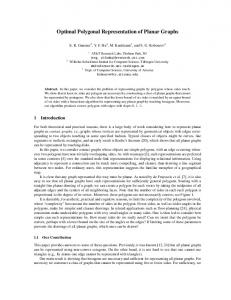
Manhattan path inside T δ (e). Next, we digitize the straight line edge e connecting u and v into a Manhattan path M (e) between u and v in the refined grid. The existence of such a Manhattan path is guaranteed by the following lemma. Lemma 5. Let e be a straight line edge connecting u and v and the length of the refined grid edge be δ/100. Then there exists a Manhattan path M (e) connecting u and v such that M (e) lies inside T δ (e). Proof. Without loss of generality, consider the edge to be of positive slope. In the refined grid, consider the grid cells that are being intersected by the straight line edge e. Since e is a straight line, two consecutive grids that are being intersected by e have the following property: the second grid cell is either to the north, or to the east or to the north-east corner of the previous grid cell as shown in Figure 5. Consider a Manhattan path M (e) from u to v that uses only
v √
√ 2δ/100
v
2δ/100
u
u Figure 5: Conversion of a straight line edge into a Manhattan path
√ those grid cells. Any point on M (e) is within a distance of 2δ/100 from the straight line edge e√because each point on a grid cell that is being intersected by the straight line edge e is within 2δ/100 distance from e. Hence, M (e) lies inside T δ (e). As discussed so far, starting from a straight line embedding of a planar graph on O(n)×O(n) grid, we have obtained an embedding of the planar graph on a refined grid of size O(n2 /δ) × O(n2 /δ) where each edge e is represented by a Manhattan path M (e). The following lemma fixes the value of δ. Lemma 6. δ = C 0 · 1/n2 , for some constant C 0 . Proof. Let δ(v) be as earlier and let it be achieved by two straight line edges vu and vw. Let A and B be the two points where the boundary of B � (v) intersects with vu and vw respectively. Hence, δ(v) = AB.
u w
A v
Q P
B
Figure 6: Fixing the value of δ in the O(n2 ) × O(n2 ) grid . Case 1: Assume that A and B are on the same side of B � (v) and both vu and vw have positive slope, as shown in the Figure 6. Let uP be the perpendicular on vw and uQ be parallel to AB. 5
Note that, vA > �/2. By Lemma 3, uP > C. So, clearly uQ > C. Since, the grid is of size O(n2 ) × O(n2 ), we have vu < C1 · n2 . Now, as 4vAB and 4vuQ are similar, we have, AB uQ �C · 1/n2 = ⇒ AB > vA vu 2C1
u A v B P
Q w
Figure 7: Fixing the value of δ in the O(n2 ) × O(n2 ) grid. Case 2: Assume that A and B are on the same side of B � (v) and vu is of positive slope and vw is of negative slope, as shown in the Figure 7. This case can be handled in a similar way. Case 3: Assume that A and B are on two consecutive sides of B � (v), as shown in the Figure 8. Let AA0 and uQ be two perpendiculars on vw. In this case, AB > AA0 . Using the similarity of 4vAA0 and 4vuQ, we have AA0 > C∈ · 1/n2 . Since AB > AA0 , we have δ(v) > C∈ · 1/n2 .
u
w
A
v
A B
Q
0
Figure 8: Fixing the value of δ in the O(n2 ) × O(n2 ) grid. Hence, by choosing an appropriate constant, we have δ = C 0 · 1/n2 for all cases. Hence, we have obtained an embedding of the planar graph on a refined grid of size O(n4 ) × O(n4 ), where each edge e is represented by a Manhattan path M (e). Also the digitization of the straight line edge is done in such a way that it avoids the corner points of B � (v). Suppose, a Manhattan path P passes through a corner point, say x, of B � (v). Consider the grid points on P that are immediately before and after x and are not on the vertical or horizontal line through x. Let these grid points be p and q. Modify the Manhattan path P by replacing the part between p and q by some other Manhattan path between p and q that does not go through x. Next, we modify the Manhattan paths inside B � (v) in the way as shown in Figure 9. While entering B � (v), if an M (e) intersects the horizontal (vertical) boundary of B � (v), the path is 6
v
v
Figure 9: Modification of M (e) inside B � (v)
altered to travel along the same horizontal (vertical) boundary of B � (v) to intersect the vertical (horizontal) grid line through v, and then follow the vertical (horizontal) grid line to v. The new path that consists of M (e) outside B � (v) and the altered path inside B � (v) is also a Manhattan path. We do this modification for all B � (v)s. Finally, we place obstacles on the four corner points of B � (v) and on all the grid points inside B � (v) except the grid points on the boundary of B � (v) and the vertical and horizontal line containing v. This is shown in Figure 9. We also place obstacles on each empty grid point outside B � (v)s. We show that this embedding is an obstacle representation of the planar graph in an O(n4 ) × O(n4 ) grid. Let us color all the paths present in the embedding into two colors, green (G) and blue (B). The portion of a path that is inside B � (v), for some v ∈ V , is colored green and all the remaining portion of the path is colored as blue. We apply this coloring technique for all the paths in the embedding. For this coloring, we have the following lemma. Lemma 7. Each Manhattan path that starts and ends at some vertices is of the form GBG, i.e., the path starts with a green portion, has a following blue portion and ends with another green portion. Proof. Let P be a path in the embedding that starts at u and ends at v. Since the starting
w
Figure 10: Path of the form GBGBG is not Manhattan and ending portion of P belongs to B � (u) and B � (v) respectively, both the end portions will be green. If there is only one blue portion in P between these starting and ending green portions, then P is of the form GBG. Hence, without loss of generality, assume that there are two blue portions. All the blue portions have to be disjoint because of Observation 4 and Lemma 5. So, there must be a green portion between these two blue portions. Hence, the path is of the form GBGBG. 7
Let the middle green portion of P belong to B � (w). Notice that according to our definition, w also acts as an obstacle. By the modification of paths inside B � (w) and the placement of the obstacles, including the corners of B � (w), it is clear that both the blue portions must touch the same side of B � (w). See Figure 10. The path can not be a straight Manhattan path also because of the corner obstacles. Hence, P can not be a Manhattan path and each Manhattan path is of the form GBG. Using this lemma, we show that each edge uv ∈ E corresponds to a Manhattan path between u and v. Lemma 8. There is an edge uv ∈ E if and only if there is a Manhattan path between u and v in the embedding. Proof. By Lemma 5, it is clear that each edge uv in the planar graph is represented by a Manhattan path M (uv) connecting u and v. Conversely, in the embedding, let us assume that there is a Manhattan path P connecting u and v. By Lemma 7, P is of the form GBG. Note that all the blue portions lie outside the �-boxes and are disjoint because of Observation 4. Hence, the blue portion of P is exactly a blue portion of some M (e). Let us now assume that the two ends of this blue portion of M (e) touch two boxes B � (u) and B � (v), respectively. This implies that e is incident to both u and v. Because of Observation 4, if a blue portion of M (e) touches some B � (v), then e is incident to v. Hence, the Manhattan path P connecting u and v in the embedding represents the edge uv ∈ E. Hence, we have the following theorem. Theorem 9. Every planar graph admits a (Z2 , `1 ) obstacle representation in O(n4 ) × O(n4 ) grid.
2.2
Embedding in Z3
In this section, we show the existence of obstacle representation in three dimension. The proof of the existential result is based on the following theorem by Pach et al. [PTT97]. Theorem 10 ([PTT97]). For every fixed r ≥ 2, any r-colorable graph with n vertices has a straight line embedding in Z3 in O(r) × O(n) × O(rn) grid. First, we construct a straight line embedding of an r-colorable graph in a refined grid such that the distance between a vertex v and a straight line edge e not containing v is sufficiently large. To do that, we give a bound on the minimum distance of a grid point from a straight line edge in the embedding that is obtained from Theorem 10. Clearly this distance is smaller than or equal to the distance of a vertex from a straight line edge. Using similar argument as in Section 2.1, we get that the minimum distance of a grid point from a straight line edge is O(1/rn), where r is the chromatic number of the graph. Now we blow the grid uniformly by a factor of C.rn such that the distance between a vertex v and a straight line edge e not containing v becomes greater than a constant C. Hence, we have the following lemma. Lemma 11. Every r-colorable graph admits a straight line embedding in O(r2 n) × O(rn2 ) × O(r2 n2 ) grid such that two vertices are at least a distance C apart and a vertex and an edge are also at least a distance C apart, where C is a constant. The idea of the proof is similar to the proof presented in Section 2.1. The idea is as follows: 1. Obtain a straight line embedding of a r-colorable graph as in Lemma 11. 2. Consider an �-cube C � (v), a cube of length �, around each vertex v such that 8
• for two distinct vertices u and v, C � (v) ∩ C � (u) = ∅, • distance between two �-cubes C � (u) and C � (v) is large (say q1 ), and • distance between an �-cube C � (v) and a straight line edge e not containing v is also adequate (at least q2 ). 3. Consider a δ-tube T δ (e) (where T δ (e) is the Minkowski sum of the embedded edge e and a disk of radius δ) around each straight line edge e such that • for each pair of disjoint straight line edges e1 and e2 , T δ (e1 ) ∩ T δ (e2 ) = ∅, • for each pair of distinct straight line edges e1 and e2 sharing a common vertex v, (T δ (e1 ) ∩ T δ (e2 )) ⊂ C � (v), and • for a vertex v and a straight line edge e not containing v, C � (v) ∩ T δ (e) = ∅. 4. Refine the grid in such a way that we can digitize the straight line edge e into a Manhattan path that lies inside T δ (e). Now, let us consider � to be � C, where C is the constant given√in Lemma 11. The value of � is chosen in such a way that both q1 = (C − �) and q2 = (C − 2�) are adequately large 1 constant. Next, we fix the δ to be a constant such that δ < 10 min{δ(v)}, where δ(v) is the v∈V
minimum Euclidean distance between consecutive intersection points of C � (v) and straight line edges e containing v. The choice of δ guarantees the following observations about C � (v) and T δ (e). Observation 12. For the particular choices of � and δ, the following properties of T δ (e) and C � (v) are true: 1. For each pair of disjoint straight line edges e1 and e2 , T δ (e1 ) ∩ T δ (e2 ) = ∅. 2. For each pair of distinct straight line edges e1 and e2 sharing a common vertex v, (T δ (e1 )∩ T δ (e2 )) ⊂ C � (v), i.e., there is no intersection between δ-tubes outside the �-cubes. 3. For a vertex v and a straight line edge e not containing v, C � (v) ∩ T δ (e) = ∅. Now refine the grid sufficiently until the length of each grid edge becomes δ/100. This is done to ensure that there are enough grid points within T δ (e) to convert the edge e into a Manhattan path inside T δ (e). The digitization of a straight line edge e connecting u and v into a Manhattan path M (e) between u and v is done in the similar way as in Lemma 5 in Section 2.1. After this step, we get an embedding of a r colorable graph in O(r2 n/δ) × O(rn2 /δ) × O(r2 n2 /δ) grid where each edge e is represented by a Manhattan path M (e). Now, for fixing the value of δ, we 0 proceed is a similar way as in Lemma 6 and we get that δ = r2Cn2 , where C 0 is a constant and r is the chromatic number of the graph. Hence, we have obtained an embedding of a r chromatic graph on a refined grid of size O(r4 n3 ) × O(r3 n4 ) × O(r4 n4 ), where each edge e is represented by a Manhattan path M (e). Also the digitization of the straight line edge is done in such a way that it avoids the edges of the cube C � (v). Next, we modify the Manhattan paths inside C � (v) in the way as shown in Figure 11. For each square face F of C � (v), let c(F ) be the point of intersection of the diagonals of F . Each Manhattan path M (e) enters the cube C � (v) through a point, say x, on some square face F of C � (v). Now, alter the portion of the Manhattan path M (e) inside C � (v) follows: (i) take any Manhattan path from x to c(F ) and then (ii) take the straight line path from c(F ) to v. We do this modification for every Manhattan paths inside C � (v). Now we place obstacles on the edges of C � (v) and everywhere inside the cube C � (v) except square faces and the axis parallel straight lines containing v. We do this modification for every cube C � (v). The Manhattan path M (e) between u and v is now modified to another path containing the altered path inside C � (u), 9
u
u
c(F )
x
x
v
v
Figure 11: Modification of a Manhattan path inside C � (v). followed by the portion of M (e) outside C � (u) and C � (v), and finally the altered path inside C � (v). Next we place obstacles on each empty grid point throughout the grid. Note that the modified paths are also Manhattan paths. Hence, we have the following theorem. Theorem 13. Every r colorable graph admits a (Z3 , `1 ) obstacle representation in O(r4 n3 ) × O(r3 n4 ) × O(r4 n4 ) grid.
2.3
Embedding in a horizontal strip
In this section, we study the `1 -obstacle representation of a graph G in a horizontal strip. A horizontal strip is a grid where the y-coordinates are bounded but the x-coordinates can be any arbitrary integer. We present a compression technique to show that every graph does not admit an `1 -obstacle representation in this case. The case of vertical strip can be argued in a similar way. Note that an `1 -obstacle representation in a horizontal strip for a graph implies its `1 -obstacle representation in Z2 . But the converse is not true. For example, Cn and Kn , for n > 4, admit `1 -obstacle representation in Z2 but not `1 -obstacle representations in horizontal strips containing only two rows. First we show that if a graph admits an `1 obstacle representation in a horizontal strip, it i1 admits an `1 -obstacle representation in a finite j3 grid. Theorem 14. Let G admit an `1 -obstacle representation in a horizontal strip of height b. Then G can have an `1 -obstacle representation in a finite grid of size b × O(b3 n).
i2
j1
Proof. Let embd(G) be the `1 -obstacle representation of G in a horizontal strip of height b. For ease of exposition, we prove the theorem i3 j2 for the case where every vertex of G has different x-coordinates in embd(G). The same arFigure 12: Maintaining the upper and lower engument holds for the case where some vertices velopes of Pi,j in T . have same x-coordinates. We say two vertices v1 and v2 are consecutive if there is no other vertex whose x-coordinate lies between the xcoordinates of v1 and v2 . If for any two consecutive vertices in embd(G), the difference between their x-coordinates is less than O(b3 ), then the theorem is immediate. Hence, we aim to prove, 10
by a compression argument, that there exists an `1 -obstacle representation of G in a horizontal strip of height b such that • the consecutive vertices of G in embd(G) remain consecutive in the new representation, and • the difference between x-coordinates of two consecutive vertices is O(b3 ). For the rest of the proof, we focus on the portion, say T of embd(G) between two consecutive vertices of G. We modify each of these portions to get a different representation of G in the same horizontal strip. The modification is as follows. Let l and r be the starting and ending vertical lines of T , respectively. Note that both l and r have b grid points each. In embd(G), there may be multiple Manhattan paths from a grid point of l to a grid point of r. Let P(i, j) denote the set of all Manhattan paths from i-th grid point of l to j-th grid point of r. In the new representation, we only maintain the upper and lower envelope of each P(i, j) and color those paths as shown in Figure 12. In T , we retain all the colored paths and put obstacles everywhere else. Let us denote this new representation by embd0 (G). Note that, in embd0 (G), the connectivity between i-th grid point of l and j-th grid point of r is maintained, if P (i, j) is non-empty. Also, putting obstacles does not create any unwanted connectivity. Hence, we have the following claim: Claim 15. The new representation embd0 (G) is an `1 -obstacle representation of G. Next we calculate the total number of bend points of embd0 (G). A bend point of embd0 (G) is a grid point on some colored path P where P changes direction. Since the height of the grid is bounded by b, the number of bend points on a colored path is at most 2b − 2. Moreover, every bend point is on some colored path that defines either an upper or a lower envelope of some P(i, j). Since there are at most O(b2 ) non-empty P(i, j)s, the total number of bend points is O(b3 ) in T . Two bend points b1 and b2 are consecutive if there is no other bend point whose x-coordinate lies between the x-coordinates of b1 and b2 . The following claim, proved later, shows that the horizontal distance between two consecutive bend points need not be arbitrarily large.
Figure 13: Illustration of compression
Claim 16. The representation embd0 (G) can be modified to another representation embd00 (G) where the number of vertical lines between two consecutive bend points is constant. So, in the representation embd00 (G), the total number of bend points is O(b3 ) and between two consecutive bend points, we have only one vertical grid line. Hence, there are O(b3 ) vertical grid lines between any two consecutive vertices. Therefore, embd00 (G) is of the size b×O(b3 n).
11
Proof of Claim 16. In embd0 (G), note that, all the colored paths that cross the section between two consecutive bend points, are horizontal. The vertical grid lines between two consecutive bend points can be compressed to only three vertical grid lines such that the first and the third vertical grid line is identical with the first and last vertical grid line of the section. In the middle grid line, we put obstacles at those y-coordinates through which there is no path that passes through the same y-coordinate in the first vertical grid line as shown in Figure 13. Repeating this process for every consecutive bend points, we have an embd00 (G) where the number of vertical lines between two consecutive bend points is constant.
3
Nonexistence of grid obstacle representation
In this section, we show that not every graph admits a grid obstacle representation1 . Let G = (V, E) be a C4 -free2 graph on more than 20 vertices having at least 8n − 19 edges. The existence of such a graph is obvious from [F96]. We will show that G has no grid obstacle representation in Z2 . A graph is called quasiplanar if it admits a drawing in a plane such that there does not exist three pairwise crossing edges. The maximum number of edges in a quasiplanar graph is 8n − 20 [AT07]. So, the graph G considered above is not quasiplanar. Theorem 17. There exists a graph that does not admit a grid obstacle representation in Z2 . Proof. Let G = (V, E) be a non-quasiplanar, C4 -free graph on more than 20 vertices having at least 8n − 19 edges. Assume that G admits a grid obstacle representation with the mapping f : V → P . Hence, for each e = (u, v) ∈ E, there is an `1 -path, say Pe , from f (u) to f (v) such that it does not encounter any obstacle. Since G is not quasiplanar, there exist three disjoint edges e1 , e2 and e3 in E such that Pe1 , Pe2 , Pe3 have a pairwise crossing. Consider the paths to be going from a point u to another point v such that the x-coordinate of u is smaller than that of v. Except for the case where both the end points of an `1 path have same y-coordinates, all the paths are either increasing (going from a point having smaller y-coordinate to a point having larger y-coordinate) or decreasing (going from a point having larger y-coordinate to a point having smaller y-coordinate). So, there must exist two paths among Pe1 , Pe2 , Pe3 such that two of them are either increasing or decreasing. Without loss of generality, assume that Pe1 and Pe2 are increasing. Let e1 = (u1 , u2 ), e2 = (v1 , v2 ) and p ∈ Z2 be a grid point where Pe1 and Pe2 cross each other. Note that, there exists an `1 path between f (u1 ) and f (v2 ) through p. The path first follows Pe1 up to the point p and then it follows Pe2 . Similarly, there is an `1 path between f (v1 ) and f (u2 ) through p. This implies that both the edges (u1 , v2 ), (v1 , u2 ) ∈ E. Note that the set {u1 , u2 , v1 , v2 } forms a C4 , which is a contradiction.
4
Hardness results Here, we study the following problem of `1 -obstacle representability of a graph.
`1 -obstacle representability on a given point set (`1 -OEPS) Instance: A graph G = (V, E) and a subset S of a polynomial sized (polynomial in |V |) grid points with |S| = |V | Question: Does there exist an `1 -obstacle representation of G such that the vertices of G are mapped to S. 1 The proof of this result was first given by J´ anos Pach [Pac16]. However, the proof presented here is different and is based on the suggestion of an anonymous reviewer of an earlier version of this paper. 2 In this case C4 -free means no subgraph of G is C4
12
Figure 14: Geodesic embedding of G0 . The black circles are original vertices and the plain circles are subdivided vertices.
Now, we show that `1 -OEPS is NP-complete for subdivision of non-Hamiltonian planar cubic graphs. The reduction is from a restricted version of geodesic point set embeddability problem. The problem is whether a planar graph has a Manhattan-geodesic drawing such that the vertices are embedded onto a given set of points S. In the restricted version of geodesic point set embeddability problem, the given point set S is partitioned into three specific sets, say P0 , P1 and P2 , where P0 = {(−j, 0)|j = 0, 1, . . . , 2n − 2}, P1 = {(j, nj)|j = 1, 2, . . . , k1 }, and P2 = {(j, −nj)|j = 1, 2, . . . , k2 } with k1 + k2 = n/2 + 1. This restricted version is known to be NP-complete [KKRW10] for subdivision of non-Hamiltonian planar cubic graphs. The formal problem statement is as follows: Restricted Manhattan-geodesic embeddability ((P0 , P1 , P2 )-GPSE) Instance: A planar graph G = (V, E) and three specific sets P0 , P1 and P2 of grid points, as mentioned above, with |P0 | + |P1 | + |P2 | = |V |. Question: Does there exist a Manhattan-geodesic embedding of G such that the vertices of G are mapped to P0 , P1 and P2 ? Theorem 18. `1 -OEPS is NP-complete for subdivision of planar cubic graphs. Proof. Note that a certificate of `1 -OEPS is a mapping f from V to S plus a set of obstacles O. Since the grid is of polynomial size, the number of obstacles is also polynomial. It is easy to see that given a certificate, we can check in polynomial time whether G realizes an `1 -obstacle representation by invoking shortest path algorithm O(n2 ) number of time. Hence, `1 -OEPS is in NP. Let G0 = (V 0 , E 0 ) be an instance of (P0 , P1 , P2 )-GPSE, i.e., G0 is a subdivision of a nonHamiltonian planar cubic graph, say G = (V, E). Note that |V | = n is even and |E| = 3n/2. Therefore, |V 0 | = 5n/2 and |E 0 | = 3n. For some k1 , k2 with k1 + k2 = n/2 + 1, let P0 = {(−j, 0)|j = 0, 1, . . . , 2n − 2}, P1 = {(j, nj)|j = 1, 2, . . . , k1 }, P2 = {(j, −nj)|j = 1, 2, . . . , k2 }, P10 = {(2j, 2nj)|j = 1, 2, . . . , k1 }, and P20 = {(2j, −2nj)|j = 1, 2, . . . , k2 }. Let S = P0 ∪ P1 ∪ P2 and S 0 = P0 ∪ P10 ∪ P20 . For such k1 , k2 with k1 + k2 = n/2 + 1, the following claim shows that `1 -OEPS is NP-complete for subdivision of planar cubic graphs. Claim 19. G0 has a Manhattan-geodesic embedding on S if and only if G0 has an `1 -obstacle representation on S 0 . Proof of Claim 19: Let G0 have a Manhattan-geodesic embedding on S (see Figure 14). From the proof of NP-hardness of GPSE [KKRW10], it follows that only vertices with degree 2 can be mapped to P1 and P2 . We can get an `1 -obstacle representation of G0 in the following way: 13
Figure 15: `1 -obstacle representation of G0 .
First, draw a row between every pair consecutive rows in the grid and then draw a column between every pair of consecutive columns in the half where the x-coordinate is non-negative. After that, place obstacles everywhere in the grid except the paths given by the Manhattangeodesic embedding of G0 (see Figure 15). Clearly, this is an `1 -obstacle representation of G0 on S0. Conversely, let G0 have an `1 -obstacle representation on S 0 . Note that, at least n − 1 vertices of degree 3 have to be mapped in P0 because otherwise two vertices of degree 2 would be consecutive in P0 , which is a contradiction to the fact that there is no edge between degree 2 vertices in G0 . Further note that, if there is a vertex of degree 3, say v, that is mapped to some point in P10 or P20 , then v has to be adjacent to the vertices that are mapped to (0, 0) and (−2n + 2, 0). This implies that G0 has a cycle of length 2n, which is a contradiction to the fact that G is non-Hamiltonian. Hence, all the vertices that are mapped to P10 and P20 , are of degree 2. Now, let p1 and p2 be two paths in the `1 -obstacle representation of G0 on S 0 between x1 , y1 and x2 , y2 respectively, where x1 , x2 ∈ P0 with {x1 , x2 } = 6 {(0, 0), (−2n + 2, 0)}, and y1 , y2 ∈ P10 . If p1 and p2 share any grid point, then there would be Manhattan path between x1 , y2 and x2 , y1 . This implies that the degree of x1 and x2 is 4, which is a contradiction. The argument also holds if y1 , y2 ∈ P20 . Note that in the case when {x1 , x2 } = {(0, 0), (−2n + 2, 0)}, we can always find another pair of points x01 , x02 ∈ P0 that will satisfy the above arguments thus leading to the aforementioned contradiction. Hence, no two paths between distinct pair of vertices share a common grid point. Given such an `1 -obstacle representation of G0 on S 0 , we can modify to get an `1 -obstacle representation of G0 on S 0 such that all the paths follow grid lines of the form x = a or y = b, where a and b are even and no two path share any grid point. In this embedding, if we delete all the rows of the form y = b0 , where b0 is odd, and delete all the columns of the form x = a0 , where a0 is any positive odd number, then we have a Manhattan embedding of G0 on S.
5
Conclusion
In this article, our main focus has been on the existential question of grid obstacle embedding of graphs in polynomial sized grids. We have proved that planar graphs admit grid obstacle representation in grids of size O(n4 ) × O(n4 ) in Z2 . The grid size may be improved by either intelligent refinement of the grid obtained in Theorem 2 or by starting with a different type of embedding of planar graph at the first place. Along this direction, the embedding studied in [FKK97] may be useful. To use this setting for grid obstacle representation of a planar graph, we have to place a vertex on a grid point inside the corresponding rectangle. But this need not produce a grid obstacle representation as there is no guarantee that all paths will 14
turn out to be Manhattan. As planar graphs admit grid obstacle representation and there exist graphs that do not, a pertinent question is to characterize the graphs that admit grid obstacle representation in Z2 . There are two associated optimality problems — given a graph G that admits `1 -obstacle representation, find the `1 -obstacle number and the minimum grid size for `1 -obstacle representation. We highlight some interesting problems in this area. Problem 1. Characterize the graphs that admit grid obstacle representation in Z2 . There are mainly two optimality problems associated with `1 -obstacle representation of a graph. The problems are as follows: Problem 2. Given a graph G that admits `1 -obstacle representation, find the `1 -obstacle number of G on Z2 . Problem 3. Given a graph G that admits `1 -obstacle representation, find the minimum grid size for `1 -obstacle representation of G on Z2 . By simple counting techniques, it can be shown that if we have a bound on the `1 -obstacle number, then there exist some graphs that can not be embedded in a small grid. This indicates a dual nature between the above two problems. Hence, the following bicriterion problem is interesting to study. Problem 4. Given a graph G that admits `1 -obstacle representation, find the representation of G on Z2 that minimizes both the grid size as well as the `1 -obstacle number.
References [AKL10] Hannah Alpert, Christina Koch, and Joshua D. Laison. Obstacle Numbers of Graphs. Discrete & Computational Geometry, 44(1):223–244, 2010. [AT07] Eyal Ackerman and G´ abor Tardos. On the maximum number of edges in quasiplanar graphs. Journal of Combinatorial Theory, Series A, 114(3):563–571, 2007. [BCV15] M. Balko, J. Cibulka, and P. Valtr. Drawing Graphs Using a Small Number of Obstacles. In Proceedings of the 23rd International Symposium on Graph Drawing and Network Visualization, GD, pages 360–372, 2015. [DM15] Vida Dujmovic and Pat Morin. On Obstacle Numbers. Electronic Journal of Combinatorics, 22(3):P3.1, 2015. [DPT09] Adrian Dumitrsecu, J´ anos Pach, and G. T´oth. A note on blocking visibility between points. Geombinatorics, 19(2):67–73, 2009. [F96] Zoltn Fredi. On the number of edges of quadrilateral-free graphs. Journal of Combinatorial Theory, Series B, 68(1):1 – 6, 1996. [FKK97] Ulrich F¨ oßmeier, Goos Kant, and Michael Kaufmann. 2-visibility drawings of planar graphs. In Proceeding of the 3rd International Symposium on Graph Drawing, GD ’96, pages 155–168, 1997. [FPP90] H. De Fraysseix, J. Pach, and R. Pollack. How to draw a planar graph on a grid. Combinatorica, 10(1):41–51, 1990. [FSS11] Radoslav Fulek, Noushin Saeedi, and Deniz Sari¨oz. Convex obstacle numbers of outerplanar graphs and bipartite permutation graphs. CoRR, abs/1104.4656, 2011.
15
[GG13] Subir Kumar Ghosh and Partha P. Goswami. Unsolved Problems in Visibility Graphs of Points, Segments, and Polygons. ACM Computing Surveys, 46(2):22, 2013. [Gho07] Subir Ghosh. Visibility Algorithms in the Plane. Cambridge University Press, 2007. [GO97] Jacob E. Goodman and Joseph O’Rourke, editors. Handbook of Discrete and Computational Geometry. CRC Press, Inc., 1997. [JS11] Matthew P. Johnson and Deniz Sari¨oz. Computing the obstacle number of a plane graph. CoRR, abs/1107.4624, 2011. [JS14] Matthew P. Johnson and Deniz Sari¨oz. Representing a Planar Straight-Line Graph Using Few Obstacles. In Proceedings of the 26th Annual Canadian Conference on Computational Geometry, CCCG, 2014. [KKRW10] B. Katz, M. Krug, I. Rutter, and A. Wolff. Manhattan-Geodesic Embedding of Planar Graphs. In Proceedings of the 17th International Symposium on Graph Drawing, GD, pages 207–218, 2010. [Mat09] Jir´ı Matousek. Blocking Visibility for Points in General Position. Discrete & Computational Geometry, 42(2):219–223, 2009. [MPP12] Padmini Mukkamala, J´ anos Pach, and D¨om¨ot¨or P´alv¨olgyi. Lower Bounds on the Obstacle Number of Graphs. Electronic Journal of Combinatorics, 19(2):P32, 2012. [MPS10] Padmini Mukkamala, J´ anos Pach, and Deniz Sari¨oz. Graphs with Large Obstacle Numbers. In Proceedings of the 36th International Workshop on Graph Theoretic Concepts in Computer Science, WG, pages 292–303, 2010. [Pac16] J´ anos Pach. Graphs with no grid obstacle representation. Geombinatorics, (2):80– 83, 2016. [PS11] J´ anos Pach and Deniz Sari¨oz. On the Structure of Graphs with Low Obstacle Number. Graphs and Combinatorics, 27(3):465–473, 2011. [PTT97] J´ anos Pach, Torsten Thiele, and G´eza T´oth. Three-dimensional Grid Drawings of Graphs. In Proceedings of the 5th International Symposium on Graph Drawing, GD, pages 47–51, 1997. [Sar11] Deniz Sari¨ oz. Approximating the Obstacle Number for a Graph Drawing Efficiently. In Proceedings of the 23rd Annual Canadian Conference on Computational Geometry, CCCG, 2011. [Sch90] Walter Schnyder. Embedding Planar Graphs on the Grid. In Proceedings of the 1st Annual ACM-SIAM Symposium on Discrete Algorithms, SODA, pages 138–148, 1990.
16