MultiAspect Graphs: Algebraic representation and algorithms arXiv ...

arXiv:1504.07893v1 [cs.DM] 29 Apr 2015

MultiAspect Graphs: Algebraic representation and algorithms Klaus Wehmuth National Laboratory for Scientific Computing (LNCC) Av. Get´ulio Vargas, 333 25651-075 – Petr´opolis, RJ – Brazil [email protected] ´ Fleury Eric LIP – UMR CNRS 5668 Ecole Normale Sup´erieure de Lyon (ENS de Lyon) / INRIA 46, alle´e d’Italie 69364 Lyon Cedex 07, France [email protected] Artur Ziviani National Laboratory for Scientific Computing (LNCC) Av. Get´ulio Vargas, 333 25651-075 – Petr´opolis, RJ – Brazil [email protected] Abstract We present the algebraic representation and basic algorithms of MultiAspect Graphs (MAGs), a structure capable of representing multilayer and time-varying networks while also having the property of being isomorphic to a directed graph. In particular, we show that, as a consequence of the properties associated with the MAG structure, a MAG can be represented in matrix form. Moreover, we also show that any possible MAG function (algorithm) can be obtained from this matrix-based representation. This is an important

1

theoretical result since it paves the way for adapting well-known graph algorithms for application in MAGs. We present a set of basic MAG algorithms, constructed from well-known graph algorithms, such as degree computing, Breadth First Search (BFS), and Depth First Search (DFS). These algorithms adapted to the MAG context can be used as primitives for building other more sophisticated MAG algorithms. Therefore, such examples can be seen as guidelines on how to properly derive MAG algorithms from basic algorithms on directed graph. We also make available python implementations of all the algorithms presented in this paper.

1

Introduction

Graph theory finds many applications in the representation and analysis of complex networked systems. In most cases, the utility of the graph abstraction comes from its inherent ability to represent binary transitive relations (i.e. transitive relations between two objects), which due to the transitivity property gives raise to key concepts, such as walks, paths, and connectivity. This graph conceptual framework allowed the emergence of basic algorithms, such as Breadth First Search (BFS) and Depth First Search (DFS) [1, 2, 3, 4, 5, 6, 7]. These basic graph algorithms, in their turn, made possible the development of more sophisticated algorithms for the analysis of specific properties of complex networks, such as network centrality or network robustness [8, 9, 10, 11], and also the analysis of dynamic processes in complex networks, such as network generative processes or information diffusion [12, 13, 14, 15, 16]. Several generalizations of the basic graph concept have been proposed for modelling complex systems that can be represented by the conjunction of distinct networks [17, 18, 19] and also complex systems in which the network itself evolves with time [20, 21, 22, 23, 24, 25, 26, 27]. More recently, further generalizations started to emerge in order to simultaneously represent the multilayer and time evolving properties [28, 29, 30, 31], although without presenting a thorough formalization, capable of justifying their basic properties. In our previous work [32], we formalize the MultiAspect Graph (MAG) structure, while also stating and proving its main properties. The structural form of the MAG presented in this previous work is similar to the multilayer structure recently presented by [30]. In both cases, the proposed structure has a construction similar to an even uniform hypergraph (i.e. the edges are composed by an even number of elements; usually greater than two). However, the adopted adjacency concept in

2

MAGs is similar to the one found in simple directed graphs, where the adjacency is expressed between two vertices, leading to a structure in which an edge represents a relation between two composite objects. Moreover, in [32], we show that MAGs are closely related to simple directed graphs, as we prove that each MAG has a simple directed graph, which is isomorphic to it. This isomorphism relation between MAGs and directed graphs is a consequence of the fact that both MAGs and directed graphs share a similar adjacency relation. MAGs find application in the representation and analysis of dynamic complex networks, such as multilayer or time-varying networks; or even networks that are both multilayer and time-varying. Examples of such networks include faceto-face in-person contact networks [33], mobile phone usage networks [34], gene regulatory networks [35], urban transportation networks [36], brain networks [37], social networks [19], among others. To illustrate the concept in more details, we present in Section 2.6 an example of modeling a simple illustrative multimodal urban transportation network. In this paper, we build upon the basic MAG properties presented in [32] and show that MAGs can be represented by matrices in a form similar to those used for simple directed graphs (i.e., those with no multiple edges). Moreover, we here show that any algorithm (function) on a MAG can be obtained from its matrix representation. This is an important theoretical result since it paves the way for adapting well-known graph algorithms for application in MAGs, thus easing the effort to develop the analysis and application of MAGs for modelling complex networked systems. We then present the most common matrix representations that can be applied to MAGs, although we do not detail all the properties of these matrices, since they are well established in the literature [7, 38, 39, 40, 41]. Further, we introduce in detail the construction of MAG algorithms for computing degree, BFS, and DFS to exemplify how MAG algorithms can be derived from traditional graph algorithms, thus providing an illustrative guideline for developing other more sophisticated MAG algorithms in a similar way. As a further contribution, we also make available python implementations of all the algorithms presented in this paper at the following URL: http://github.com/wehmuthklaus/ MAG_Algorithms. This paper is organized as follows. Section 2 briefly presents the basic MAG definitions and properties derived from [32] in order to allow enough background of the current paper. Section 2 also presents illustrative examples of MAGs and its adjacency notion. Section 3 shows the representation of MAGs by means of algebraic structures, such as tensors and matrices. Emphasis is given to matrix representations, which are derived from the isomorphism relation between MAGs 3

and simple directed graphs. In particular, we also introduce in Section 3.1 the companion tuple, which is a complement to the MAG matrix representations. In Section 4 we present basic MAG algorithms which are derived from well-known simple graph algorithms. Further, in Section 4.2, we show that any algorithm (function) that can be defined for a MAG can be also obtained from its adjacency matrix and companion tuple, establishing the theoretical basis for deriving MAG algorithms from well-known simple graph algorithms. Finally, Section 5 presents our final remarks and perspectives for future work.

2

MultiAspect Graph (MAG)

In this section, we present a formal definition of a MAG, as well as some key properties, which are formally stated and proved in [32].

2.1

MAG definition

We define a MAG as H “ pA, Eq, where E is a set of edges and A is a finite list of aspects. Each aspect ϕ P A is a finite set, and the number of aspects p “ |A| is called the order of H. Each edge e P E is a tuple with 2 ˆ p elements. All edges are constructed so that they are of the form pa1 , . . . , a p , b1 , . . . , b p q, where a1 , b1 are elements of the first aspect of H, a2 , b2 are elements of the second aspect of H, and so on, until a p , b p which are elements of the p-th aspect of H. Note that the ordered tuple that represents each MAG edge is constructed so that their elements are divided into two distinct groups, each having exactly one element of each aspect, in the same order as the aspects are defined on the list A. As a matter of notation, we say that ApHq is the aspect list of H and EpHq is the edge set of H. Further, ApHqrns is the n-th aspect in ApHq, |ApHqrns| “ τn is the number of elements in ApHqrns, and p “ |ApHq| is the order of H. In addition to the former definition, we define the following two sets constructed from the cartesian products of aspects of an order p MAG: p ą

VpHq “

ApHqrns,

(1)

n“1

the cartesian product of all the aspects of the MAG H, and 2p ą

EpHq “

ApHqrpn ´ 1qpmod pq ` 1s,

n“1

4

(2)

which is the set of all possible edges in the MAG H, so that EpHq Ď EpHq. We call u P VpHq a composite vertex of MAG H. As a matter of notation, a composite vertex is always represented as a bold lowercase letter, as in u, for instance. From the properties stated for the MAG edge in our definition, it follows that an MAG edge is closely related to an ordered pair of composite vertices. For any given MAG H, every MAG edge e P EpHq has the form pa1 , . . . , a p , b1 , . . . , b p q, so that pa1 , . . . , a p q P VpHq and pb1 , . . . , b p q P VpHq are composite vertices of this given MAG H. From this, we can define two functions πo : EpHq Ñ VpHq e “ pa1 , a2 , . . . , a p , b1 , b2 , . . . , b p q ÞÑ pa1 , a2 , . . . , a p q “ u,

(3)

πd : EpHq Ñ VpHq e “ pa1 , a2 , . . . , a p , b1 , b2 , . . . , b p q ÞÑ pb1 , b2 , . . . , b p q “ v.

(4)

and

We call πo peq the origin composite vertex of e and πd peq the destination composite vertex of e. Moreover, we can define the function ą ψ : EpHq Ñ VpHq VpHq (5) e ÞÑ pπo peq, πd peqq “ ppa1 , . . . , a p q, pb1 , . . . , b p qq “ pu, vq, from which we can construct a directed graph GH “ pV pHq, ψpEpHqq. In [32], we demonstrate that the directed graph GH “ pV pHq, ψpEpHqq is isomorphic to the MAG H from which it was originated. At this point, we can therefore define the function ą g : pApHq, EpHqq Ñ pVpHq, VpHq VpHqq (6) H ÞÑ pVpHq, ψpEpHqq, which maps every MAG H to its isomorphic directed graph gpHq. Further, we define the set of functions πi : VpHq Ñ ApHqris pa1 , a2 , . . . , a p q ÞÑ ai , which extracts the n-th element of a composite vertex tuple. 5

(7)

2.2

MAG sub-determination

The sub-determination is a generalization of the aggregation concept applied to multilayer or time-varying graphs, in which all layers can be aggregated, resulting in a traditional graph. Since a MAG can have more than 2 aspects, the subdetermination can be done in more ways than the aggregation. Given an arbitrary MAG H, a sub-determination is constructed from a nonempty proper sublist of the aspects of H. Since this sublist excludes the empty sublist and the full aspects list of H, in a MAG with p aspects there are 2 p ´ 2 possible non-empty proper aspect sublists, each one of them originating a distinct sub-determination. Therefore, in a MAG H with p aspects we identify the possible sub-determination by a positive integer ζ , where 1 ď ζ ď 2 p ´ 2. A tuple with p elements either 0 or 1 can be used to represent each possible sub-determination. An element with value 1 in the i-th position of the tuple indicates that the i-th aspect is present in the sub-determination, while a 0 indicates that the i-th aspect is not present in the sub-determination. We remark that this tuple coincides with the binary representation of the integer ζ . We therefore use the symbol ζ to represent the sub-determination both as an integer number or its equivalent tuple. For a given MAG H and a sub-determination ζ , we have a sublist Aζ pHq Ă ApHq such that pζ “ |Aζ pHq| is the number of aspects in the sub-determination. From this, we define the set of composite sub-determined vertices of H as pζ ą

Vζ pHq “

(8)

Aζ pHqrns,

n´1

the cartesian product of all the aspects present on the sub-determination list. Further, we define the function Sζ : VpHq Ñ Vζ pHq

(9)

pa1 , a2 , . . . , a p q ÞÑ paζ1 , aζ2 , . . . , aζ p q, ζ

which takes each composite vertex of H to its sub-determined form.

2.3

MAG adjacency

Two composite vertices are considered adjacent if they share the same MAG edge, i.e. given two composite vertices u, v P VpHq are adjacent if and only if there is a MAG edge e P EpHq such that u, v P tπo peq, πd pequ. Similarly, two MAG edges 6

are considered adjacent if and only if they share a same composite vertex, i.e. two given edges e1 , e2 P EpHq are adjacent if and only if there is a composite vertex u P VpHq such that u P tπo pe1 q, πd pe1 qu and u P tπo pe2 q, πd pe2 qu. Figure 1 shows an illustrative example of three MAG edges. The figure depicts a four aspects MAG, where each set of colored circles represents one aspect, and each edge has two elements of each aspect.

Figure 1: Illustrative example of three MAG edges. The isolated edge pA1, A2, A3, A4,C1,C2,C3,C4q on the leftmost side of Figure 1 exemplifies the composite vertex adjacency concept. In this case the composite vertices pA1, A2, A3, A4q and pC1,C2,C3,C4q are adjacent. The two edges pE1, E2, E3, E4, H1, H2, H3, H4q and pH1, H2, H3, H4, K1, K2, K3, K4q exemplify a case of edge adjacency. Since the composite vertex pH1, H2, H3, H4q is shared by both edges, they are adjacent. Although the structure of a MAG edge is similar to an even uniform hypergraph edge, the adjacency definition used on MAGs is not the usual one adopted 7

on hypergraphs. The adjacency concept found on a MAG is close to the one associated with traditional directed graphs, where a MAG edge can be seen as a relation between two composite vertices, which are composite objects constructed from aspect elements. Therefore, a MAG edge expresses a relationship between two (composite) objects in the same way as a directed graph edge. This concept leads to the isomorphism between MAGs and directed graphs, as well as the close relation between walks, trails, and paths on MAGs and directed graphs.

2.4

MAG isomorphism

Two MAGs of order p, H and K, are isomorphic if p “ |ApHq| “ |ApKq|, there is a permutation σ such that for 1 ď i ď p we have that |ApHqris| “ |ApKqrσ piqs|, and there is a bijective function f : VpHq Ñ VpKq such that an edge e P EpHq if and only if there is an edge p f pπo peqq, f pπd peqqq P EpKq. This is to say that the two MAGs are isomorphic if they have the same order, the aspects of one are a permutation of the aspects of the other, and there is a bijective function between the composite vertices sets that preserves the adjacency on the MAGs. Since isomorphism is an equivalence relation, we can use it to partition the set of all MAGs with finite set of composite vertices. Therefore, let « be the MAG isomorphism relation, and H the set of all MAGs with finite composite vertices set. We then define H “ H { «, the quotient set of all finite MAGs under the isomorphism relation. Each element of H is an equivalence class containing isomorphic MAGs. Therefore, H P H is a MAG that represents a class of MAGs isomorphic to it.

2.5

MAG walks, trails, and paths

There is a close relation between walks, trails, and paths on a MAG and their counterparts in the isomorphic directed graph gpHq. A walk on a MAG H is defined as an alternating sequence W “ ru1 , e1 , u2 , e2 , u3 , . . . , uk´1 , ek´1 , uk s of composite vertices un P VpHq and edges em P EpHq, such that un “ πo pen q and un`1 “ πd pen q for 1 ď n ă k. It follows from this definition that in a walk, consecutive composite vertices as well as consecutive MAG edges are adjacent. We show in [32] that an alternating sequence W of composite vertices and edges in a MAG H is a walk on H if and only if there is a corresponding walk GW in the composite vertices representation of H. This means that a walk on a MAG H has a isomorphic walk on the directed graph gpHq. Since trails and paths 8

also are walks, we also show that the same isomorphism concept extends to them as well. Figure 1 can also exemplify a MAG path. The two edges pE1, E2, E3, E4, H1, H2, H3, H4q and pH1, H2, H3, H4, K1, K2, K3, K4q can also be seen as part of the alternating sequence P “ pE1, E2, E3, E4q, pE1, E2, E3, E4, H1, H2, H3, H4q, pH1, H2, H3, H4q, pH1, H2, H3, H4, K1, K2, K3, K4q, pK1, K2, K3, K4q, which characterizes a two-hops path from the composite vertex pE1, E2, E3, E4q to the composite vertex pK1, K2, K3, K4q. From the concept that walks, trails, and paths on a MAG have a isomorphism relation to their counterparts on the directed graph gpHq, it follows that analysis and algorithms based on walks, trails, and paths can be formulated on the directed graph gpHq. These properties will be extensively used in the current work.

2.6

MAG example

Figure 2 shows an example of a three aspect MAG T . It can be seen as the representation of a time-varying multilayer network, showing a small and simplified section of an urban transportation system. More specifically, Figure 2 depicts the MAG T in its composite vertices representation, gpT q, which is the directed graph defined in Equation (6). A detailed derivation of this representation can be found in [32]. Aligned with this view, the aspects of MAG T can be interpreted in the following way: The first aspect represents three distinct locations, labeled 1, 2 and 3. Specifically, location 1 represents a subway station, location 2 a subway station with a bus stop, and location 3 a bus stop. The second aspect represents two distinct urban transportation modes depicted as layers, namely Bus and Subway. Finally, the third aspect represents three time instants. The MAG edges can be seen with the following meaning: Location 1 has no edges on the bus transportation mode, since it is a subway station. Similarly, location 3 has no edges on the subway mode, since it is a bus stop. The six blue (dashed) edges show that it is possible to change between bus and subway layers at all times at location 2. As a simplification, the connection between the bus and subway layers is assumed to take no time. The eight black edges represent bus and subway trips between locations. As a simplification all trips are assumed to have the same duration. The red (dotted) edges represent the possibility of staying at a bus stop or subway station and not taking a transport. In this model, walks represent the ways the urban transportation system can be used to travel from one location to another. For instance, starting at location 1 9

Figure 2: Illustrative MAG T of a simple urban transportation system. on the subway layer at time t1, it is possible to reach location 3 on the bus layer at time t3. It can be done by taking a subway trip to location 2 at time t2, switching from subway to bus layer at location 2, time t2 and finally taking a bus trip from location 2 bus layer arriving at location 3 on the bus layer at time t3. The presence of unconnected occurrences of location 1 at bus layer and location 3 at subway layer can be viewed as artefacts of the MAG construction. We call these vertices trivial components of the MAG. This subject will be further later addressed on this paper. The MAG example shown in Figure 2 will be used in this work to provide simple illustrative examples where needed.

3

Algebraic Representation

In this section, we discuss ways to represent MAGs by means of algebraic structures. Due to the format of the MAG edge and its similarity to an even uniform 10

hypergraph, it is straightforward to construct tensorial algebraic representations for MAGs. Nevertheless, as a consequence to the isomorphism between MAGs and traditional directed graphs, it is also possible to have matrix-based representations of MAGs. This section addresses both types of representations, using the MAG depicted in Figure 2 as an illustrative example. In this work, we consider a tensor to be a multi-dimensional array of entries, which in other previous works is also called a hypermatrix. Further, we reserve the denomination tensor for arrays whose dimension is above 2. Dimension 2 arrays are called matrices and dimension 1 arrays are called vectors. A matrix with the same number of elements in each of its two dimensions is called a square matrix, whereas a tensor with the same number of elements in all of its dimensions is called a hypercubical tensor.

3.1

Companion tuple

Although we show in [32] that every MAG H is isomorphic to a directed graph designated gpHq, it is important to note that the set of vertices of this graph is VpHq, as shown in Equation (6). Since the set VpHq is the cartesian product of all the aspects in the MAG H, it is possible to reconstruct the MAG’s aspect list from VpHq, which is a step necessary to obtain the MAG H from the directed graph gpHq. When the vertices of the directed graph G associated with a given MAG H are not the composite vertices themselves, it is necessary to provide a mechanism to link each vertex of the directed graph to its corresponding composite vertex on the MAG. This mechanism can be, for instance, a bijective function between VpHq and V pGq. In the current work, we construct representations for gpHq, such as matrices, which do not directly carry the tuples that characterize the MAG’s composite vertices. In this kind of representation, a vertex is associated with a row or column of a matrix. Therefore, additional information has to be provided in order to properly link each row (column) of a matrix to its corresponding composite vertex on the MAG represented by this matrix. This is done by a bijective function D, defined in Section 3.2, where D takes a composite vertex to a natural number, which is the row (column) number in the matrix. The implementation of D presented in this work is based on the concept of a companion tuple, which complements the matrix representation of a given MAG. For a MAG H with p aspects, its companion tuple has the form p|ApHqr1s|, |ApHqr2s|, . . . , |ApHqrps|q, so that the number of elements on it equals the order of H and each element represents the number of elements of an aspect of H. As a 11

matter of notation, we represent the companion tuple of a given MAG H as τpHq “ p|ApHqr1s|, |ApHqr2s|, . . . , |ApHqrps|q,

(10)

where p is the order of H. When there is no ambiguity in relation to which MAG we are referring to, we may use the notation τ instead of τpHq. For instance, the companion tuple of the MAG T shown in Figure 2 is τpT q “ p3, 2, 3q, since T has 3 aspects, of which the first has 3 elements, the second 2 elements, and the third 3 elements. Algorithm 1 shows the building of the companion tuple for a given MAG H. Assuming that the size of the aspect list ApHq and the size of each of the aspect sets contained in ApHq are known from the computational representation of ApHq, the time complexity for building the companion tuple is Oppq, where p is the number of aspects on MAG H. If, however, these sizes are unknown, then the řp time complexity is Opsq, where s “ i“1 |ApHqris|, since each element of each aspect has to be counted. We remark that, in either case, the time complexity for building the companion tuple is less than OpVpHqq, which is the order of the set of composite vertices of the MAG. input : ApHq output: τpHq CompTuple(ApHq) p Ð |ApHq| // number of aspects in the MAG 3 for i Ð 1 to p do 4 T ris Ð |ApHqris| // number of elements in i-th aspect 5 end 6 return T Algorithm 1: Construction of the companion tuple of a MAG.

1

2

For a given MAG H and a sub-determination ζ , we also define the subdetermined companion tuple τζ pHq, which is obtained by multiplying each entry of the original companion tuple by the equivalent entry of the tuple representation of ζ , as shown in Algorithm 2. The sub-determined companion tuple has the same value as the original companion tuple for the aspects that have value 1 in ζ and 0 otherwise.

12

input : τpHq, ζ output: τζ pHq SubCompTuple(τpHq, ζ ) p Ð |τpHq| // number of aspects in the MAG 3 for i Ð 1 to p do 4 Tζ ris Ð τpHqris ˚ ζ ris 5 end 6 return Tζ Algorithm 2: Construction of sub-determined companion tuple. 1 2

3.2

Order of composite vertices and aspects

In general, the order of the composite vertices and aspects on a MAG is not relevant. That is, changing the order in which the aspects or their elements are presented does not affect the result of any algorithm or analysis performed on a MAG, since the MAG obtained by such changes is isomorphic to the original one. The definition of the MAG isomorphism adopted in this work can be found in Section 2.4. However, in order to show the MAG’s algebraic representation in a consistent way, it is necessary to link the MAG’s composite vertices to rows and columns of matrices, which is achieved by the bijective function D, defined in this section at Equation (12). We now show the preliminary steps necessary for the definition of function D, as implemented in this work. The aspect order is adopted as the same in which the aspects are placed on the MAG’s companion tuple. For the ordering of composite vertices, we define the numerical representation of each composite vertex from its tuple. In order to obtain the composite vertex numerical representation, we first translate the composite vertex into a numerical tuple. This is done by applying a family of indices, one for each aspect on the composite vertex, where for every aspect i the corresponding index ranges from 0 to τi ´ 1, where τi is the number of elements on the i-th aspect of the MAG. Since this is a simple index substitution, we do not use a distinct notation for the composite vertex on its numerical tuple form. We, however, reserve the notation uris to express the i-th element of the composite vertex on its numerical form. To calculate the numerical representation of a composite vertex, we define the weight of each position on the composite vertex tuple of a MAG H with p aspects

13

as

" W pi, τq “

1 śi´1

j“1 τ j

if i “ 1, otherwise,

(11)

where i is the position in the tuple varying from 1 to p, τ is the MAG’s companion tuple, and τ j is the j-th element of the MAG’s companion tuple. Note that |τ| “ p meaning that the length of the companion tuple is the order of the MAG, i.e. the number of its aspects. Finally, we define the composite vertex numerical representation as |τ| ÿ (12) Dpu, τq “ 1 ` W pi, τq ˆ uris, i“1

where |τ| “ p is the MAG’s order, and vris is the i-th component of the composite vertex. Figure 3 shows the MAG T with its composite vertices, and their numerical representations ranging from p1q to p18q. In order to illustrate how the numerical representations are obtained, we show examples based on the MAG T . For this representation, we adopt aspect indices such that for aspect 1 we have Idxp1q “ 0, Idxp2q “ 1 and Idxp3q “ 2. For aspect 2, we have IdxpBusq “ 0 and IdxpSubwayq “ 1, while for aspect 3, Idxpt1 q “ 0, Idxpt2 q “ 1 and Idxpt3 q “ 2. Since the companion tuple of MAG T is τpT q “ p3, 2, 3q “ τ, the weights are W p1, τq “ 1, W p2, τq “ τ1 “ 3 and W p3, τq “ τ1 ˆ τ2 “ 6. Therefore, the composite vertex v “ p1, Bus,t1 q has numerical representation Dpv, τq “ 1 ` 1 ˆ 0 ` 3 ˆ 0 ` 6 ˆ 0 “ 1, while Dpp2, Subway,t2 q, τq “ 1 ` 1 ˆ 1 ` 3 ˆ 1 ` 6 ˆ 1 “ 11 and Dpp2, Bus,t3 q, τq “ 1 ` 1 ˆ 1 ` 3 ˆ 0 ` 6 ˆ 2 “ 14. Algorithm 3 determines the numerical representation of a composite vertex v represented by its numerical tuple. The presented implementation extends the concepts presented in Equations (11) and (12), so that this algorithm can also be used to determine the numerical representation of sub-determined composite vertices. In order to determine the numerical representation of a sub-determined vertex, function D shown in Algorithm 3 receives the full composite vertex tuple (not sub-determined) and the sub-determined companion tuple. The if seen at line 7 of Algorithm 3 makes that the 0 entries found in a sub-determined companion tuple are discarded for the construction of the sub-determined numerical representation of the composite vertex. The time complexity for this algorithm is Oppq, where p is the number of aspects on the MAG in question. Given the numerical representation of any composite vertex, it is possible to reconstruct its tuple. In order to do this, we calculate the numerical value of the

14

Figure 3: MAG T with composite vertices numerical representations index of each element on the tuple, as Npd, i, τq “ tppd ´ 1q mod W pi ` 1, τqq { W pi, τqu,

(13)

where d is the composite numerical representation, i is the position of the composite vertex tuple to be calculated, τ is the MAG’s companion tuple, mod is the modulus (division remainder) operation and txu is the floor operator, which for any x P R corresponds to the largest integer i P Z such that i ď x. Note that for calculating Npd, p, τq for a MAG with p aspects, it is necessary to calculate W pp ` 1, τq. Considering the definition of W from Equation (11), it follows that ś W pp ` 1, τq “ pj“1 “ |VpHq|, the number of composite vertices on the MAG. For instance, taking the composite vertex with numerical representation 14 of

15

input : v, τpHq output: d // v is the numerical tuple of the composite vertex

1

D(v, τpHq) p Ð |τpHq| // number of aspects in the MAG 4 dÐ0 5 wÐ1 6 for i Ð 1 to p do 7 if τpHqris ‰ 0 then 8 d Ð d ` pvris ˚ wq 9 w Ð w ˚ τpHqris 10 end 11 end 12 return d Algorithm 3: Determination of the numerical representation of a composite vertex. 2

3

the MAG T , we have that Np14, 1, p3, 2, 3qq “tpp14 ´ 1q mod 3q{1u “ t1{1u “ 1 Np14, 2, p3, 2, 3qq “tpp14 ´ 1q mod 6q{3u “ t1{3u “ 0 Np14, 3, p3, 2, 3qq “tpp14 ´ 1q mod 18q{6u “ t13{6u “ 2.

We can therefore define the inverse of function D as D´1 pd, τq “ pNpd, 1, τq, Npd, 2, τq, . . . , Npd, |τ|, τqq,

(14)

which reconstructs the composite vertex tuple in its numerical form. From this, we can see that, for instance, D´1 p14, p3, 2, 3qq “ p1, 0, 2q, which corresponds to the composite vertex p2, Bus,t3 q. Algorithm 4 shows the implementation of D´1 . The relation between the composite vertex numerical representation and its tuple can also be seen as a consequence of the isomorphism between the MAG H and its composite vertices representation, gpHq. The role of this relation will become clear in Sections 3.6 to 3.8, where the matrix forms of the MAG are presented. 16

input : d, τpHq output: v 1

// v is the numerical tuple of the composite vertex

InvD(d, τpHq) p Ð |τpHq| // number of aspects in the MAG 4 wr1s Ð 1 5 wl Ð 1 6 for i Ð 1 to p do 7 if τpHqris ‰ 0 then 8 wri ` 1s Ð wris ˚ τpHqris 9 wl Ð wl ` 1 10 end 11 end 12 for i Ð 1 to wl do 13 vris Ð pd Mod wri ` 1sq{wris 14 end 15 return v Algorithm 4: Determination of the composite vertex from its numerical representation. 2

3

3.3

Elimination of trivial components

In the MAG T shown in Figure 3 the composite vertices of numerical representation p1q, p6q, p7q, p12q, p13q, and p18q are trivial components (i.e. unconnected composite vertices). They are created in consequence of the regularity needed on the MAG to make it possible for it to be represented algebraically by tensors, as shown in Sections 3.4 and 3.5. This type of padding is not necessary in the directed graph and its algebraic representation. Therefore, it is possible to remove the trivial components from the composite vertices representation and its associated matrices. However, it is important to bear in mind that the graph resulting of this transformation may no longer be isomorphic to the MAG and neither are the matrices associated with it. The only case in which the isomorphism is preserved is when there are no trivial components on the MAG and nothing is removed. Nevertheless, this kind of transformation can be helpful for application, by reducing the number of composite vertices present on the graph and so simplifying its construction and manipulation. The same sort of padding is discussed in [30], where authors suggest that this 17

padding may cause problems in the computing of some metrics, such as mean degree or clustering coefficients, unless one accounts for the padding scheme in an appropriate way. In this subsection, we show that the padding with the trivial components may be eliminated, if desired. Anyway, if needed, it suffices to be cautious in computing the metrics of interest on MAGs by considering the existence of the padding scheme, as suggested by [30]. In particular, the MAG algorithms we discuss in Section 4 remain unaffected by this padding issue. For a given MAG H, we define its main components graph mpHq as the MAG’s composite vertices representation with all its trivial components removed. Figure 4 shows the main components graph mpT q for the MAG T . It is worth noting that numerical representations are not defined for mpT q.

Figure 4: mpT q of the example MAG T This can be achieved algebraically for any MAG H with the help of a matrix RpHq constructed from the identity I P Rnˆn , where n “ |VpHq| is the number of composite vertices on the MAG. The matrix RpHq is obtained from this n ˆ n identity by removing the columns which match the numerical representations of the trivial components of the MAG. Therefore, assuming that the MAG H has r trivial components, the matrix RpHq P Rnˆn´r has n rows and n ´ r columns. In particular, in the cases where the MAG H has no trivial components, we have that RpHq “ I P Rnˆn . It is also worth noting that the matrix Im pHq “ RpHq RpHqT P Rnˆn is a matrix akin to the identity I P Rnˆn , but the diagonal entries corresponding to the 18

trivial components (removed in RpHq) have value 0. Therefore, multiplying a n ˆ n matrix by Im pHq to the left has the effect of turning all entries on the rows corresponding to the trivial components to 0s. Similarly, multiplying by Im pHq to the right has the effect of turning the entries of the columns corresponding to the trivial elements to 0s. As an example, we show the matrix RpT q P R18ˆ12 , » fi 0 0 0 0 0 0 0 0 0 0 0 0 —1 0 0 0 0 0 0 0 0 0 0 0ffi — ffi —0 1 0 0 0 0 0 0 0 0 0 0ffi — ffi —0 0 1 0 0 0 0 0 0 0 0 0ffi — ffi —0 0 0 1 0 0 0 0 0 0 0 0ffi — ffi —0 0 0 0 0 0 0 0 0 0 0 0ffi — ffi —0 0 0 0 0 0 0 0 0 0 0 0ffi — ffi —0 0 0 0 1 0 0 0 0 0 0 0ffi — ffi —0 0 0 0 0 1 0 0 0 0 0 0ffi — ffi , RpT q “ — (15) ffi 0 0 0 0 0 0 1 0 0 0 0 0 — ffi —0 0 0 0 0 0 0 1 0 0 0 0ffi — ffi —0 0 0 0 0 0 0 0 0 0 0 0ffi — ffi —0 0 0 0 0 0 0 0 0 0 0 0ffi — ffi —0 0 0 0 0 0 0 0 1 0 0 0ffi — ffi —0 0 0 0 0 0 0 0 0 1 0 0ffi — ffi —0 0 0 0 0 0 0 0 0 0 1 0ffi — ffi –0 0 0 0 0 0 0 0 0 0 0 1fl 0 0 0 0 0 0 0 0 0 0 0 0 which is obtained from the 18 ˆ 18 identity matrix by removing the columns 1, 6, 7, 12, 13, and 18 that correspond to the trivial components of the MAG T .

3.4

Adjacency tensor

Since on a p aspects MAG every edge is an ordered tuple with 2p entries, it is straightforward to represent a MAG by means of an order 2p adjacency tensor. We define the adjacency tensor J pHq P Rτ1 ˆ¨¨¨ˆτ p ˆτ1 ˆ¨¨¨ˆτ p so that for each entry " 1 if p j1 , . . . , j2p q P EpHq, j j1 ,..., j2p “ (16) 0 otherwise, where τi “ |ApHqris| is the number of elements present on the i-th aspect of the MAG H. Note that τi also corresponds to the i-th entry of the companion tuple of 19

the MAG H. The tensor J pHq has its dimension (i.e. the number of entries) determined by the companion tuple of the MAG, such that for a given MAG H with p aspects, ˜ p ¸2 ź |J pHq| “ τi .

(17)

i“1

The number of elements present on each aspect of a MAG are not necessarily the same, as can be seen on the MAG T shown in Figure 2, where the aspects have 3, 2, and 3 elements, respectively. Therefore, in general, the adjacency tensor of a MAG may not be hypercubical. In consequence, eigenvalues and eigenvectors can not be determined for MAG adjacency tensors [42]. Although it is possible to determine singular values for this kind of tensors, as shown in [42], the analysis of these properties will not be pursued in this particular work. The adjacency tensors of MAGs found in practical applications are usually sparse, in the sense that the number of non-zero entries is small compared to the number of entries on the tensor. For instance, considering the 3 aspects MAG T shown in Figure 2, it has three aspects, where the first has 3 elements, the second 2 elements and the third 3 elements. ś Therefore, the order of the adjacency tensor of T is 6 and its dimension is p 3i“1 τi q2 “ p3 ˚ 2 ˚ 3q2 “ 182 “ 324. Since T has 22 edges, it follows that only 22 of the 324 entries on the tensor J pT q will be non-zero.

3.5

Incidence tensor

Considering that a given MAG H has p aspects and m edges it is also possible to construct an algebraic representation by means of an order p ` 1 tensor whose coordinates correspond to the edges and each aspect. We define the incidence tensor C pHq P Rmˆτ1 ˆ¨¨¨ˆτn for which each entry $ & ´1 if p j1 , . . . , j p q “ πo peq, 1 if p j1 , . . . , j p q “ πd peq, ce, j1 ,..., j p “ (18) % 0 otherwise, where πo peq are the origin elements of the edge e P EpHq, πd peq are the destination elements of the edge e P EpHq, m “ |EpHq| is the number of edges on MAG H, and τi “ |ApHqris| is the number of elements present on the i-th aspect of the

20

MAG H. The number of elements on the incidence tensor C pHq is |C pHq| “ m ˆ

p ź

τi .

(19)

i“1

As with the adjacency tensor, the incidence tensor is also usually sparse and, in general, not hypercubical. Considering the ś pMAG T depicted in Figure 2, its incidence tensor C pT q P R22ˆ3ˆ2ˆ3 has m ˆ i“1 τi “ 22 ˆ 3 ˆ 2 ˆ 3 “ 396 entries, of which 2 ˆ m “ 44 are not zero.

3.6

Adjacency matrix

As a direct consequence of the isomorphism between MAGs and traditional directed graphs [32], which stems from the adjacency notions used on MAGs, it is expected that a MAG can be represented in matrix form. In fact, such representations can be achieved directly by the composite vertices representation of MAGs, presented in Section 2.1. Since for any given MAG H its composite vertices representation is a traditional directed graph, it can be represented in matrix form. One of such representations is the MAG’s adjacency matrix. This matrix is obtained from the MAG’s composite vertices representation, gpHq, and its companion tuple τpHq. In fact, the MAG’s adjacency matrix is the adjacency matrix of the composite vertices representation, where the order of the rows and columns is given by the numerical representation of the composite vertices of gpHq. The set VpHq of composite vertices of a given MAG H is obtained by the cartesian product of all aspects of the MAG, as shown in Equation (1). Therefore, the number of composite vertices on a given MAG H with p aspects is n “ |VpHq| “

p ź

τi ,

(20)

i“1

where τi is the i-th element of the MAG’s companion tuple, i.e. the number of elements on the MAG’s i-th aspect. Hence, the MAG’s adjacency matrix JpHq P Rnˆn has the same number of entries as its adjacency tensor J pHq. The general form of any entry of the matrix JpHq is given by " 1 if pu, vq P EpgpHqq, ju,v “ (21) 0 otherwise, where pu, vq P EpgpHqq means that pu, vq is an edge on the composite vertices representation gpHq of the MAG H, so that u, v P VpHq are composite vertices 21

of H. It follows from the definition of gpHq and its isomorphism to H (shown in [32]), that pu, vq P EpgpHqq if and only if there is an edge e P EpHq such that u “ πo peq and v “ πd peq. Since for each edge e “ p j1 , . . . , j2p q P EpHq there is exactly one edge pu, vq P EpgpHqq such that u “ p j1 , . . . , j p q “ πo peq and v “ p j p`1 , . . . , j2p q “ πd peq, it follows that every entry ju,v “ 1 in JpHq corresponds to exactly one entry j j1 ,..., j2p “ 1 in the tensor J pHq. Therefore, the adjacency matrix JpHq can be seen as a matrization [43] of the adjacency tensor J pHq for every MAG H. This property of the adjacency matrix is a consequence of the isomorphism between the MAG H and its composite vertices representation gpHq. It is important to note, however, that the notation ju,v is in fact a shorthand for jDpu,τq,Dpv,τq , where Dpu, τq is the row number and Dpv, τq the column number of the matrix entry. This ties the construction of the adjacency matrix of a MAG with its companion tuple, since it is used in the determination of the numerical representation of a composite vertex (Dpu, τq). Therefore, the adjacency matrix of any given MAG is always presented with its companion tuple. The adjacency matrix of a given MAG H is constructed by Algorithm 5, where |VpHq| is the number of composite vertices in H, which can be calculated using Equation (20), Dpπo peq, τq and Dpπd peq, τq are the numerical representation of the origin and destination composite vertices of edge e P EpHq, respectively, as defined in Section 3.2. Considering that a sparse matrix with all entries 0 can be creinput : H “ pA, Eq output: JpHq, τpHq 1 2 3 4 5 6 7 8 9 10

AdjMatrix(H) n Ð |VpHq| T Ð CompTuplepApHqq // companion tuple JpHq Ð n ˆ n matrix with all entries “ 0 for each e P EpHq do u Ð Dpπo peq, T q // numerical origin v Ð Dpπd peq, T q // numerical destination JpHqru, vs Ð 1 end return JpHq, T Algorithm 5: Building JpHq from MAG H.

ated in constant time, and that both functions CompTuple and D (see Algorithm 1 and Algorithm 3) have time complexity Oppq, we conclude that Algorithm 5 has 22

time complexity Opp ˚ |EpHq|q, where p is the number of aspects of MAG H and |EpHq| the number of edges. As an example, the adjacency matrix of the MAG T is shown in Equation (22). This adjacency matrix JpT q P R18ˆ18 has 324 entries, of which just 22 are nonzero. It is a matrization of the adjacency tensor J pT q P R3ˆ2ˆ3ˆ3ˆ2ˆ3 , with the same number of entries and non-zero entries, reflecting the isomorphism between the MAG T and its composite vertices representation gpT q. » — — — — — — — — — — — — JpT q “ — — — — — — — — — — — — –

0 0 0 0 0 0 0 0 0 0 0 0 0 0 0 0 0 0

0 0 0 0 1 0 0 0 0 0 0 0 0 0 0 0 0 0

0 0 0 0 0 0 0 0 0 0 0 0 0 0 0 0 0 0

0 0 0 0 0 0 0 0 0 0 0 0 0 0 0 0 0 0

0 1 0 0 0 0 0 0 0 0 0 0 0 0 0 0 0 0

0 0 0 0 0 0 0 0 0 0 0 0 0 0 0 0 0 0

0 0 0 0 0 0 0 0 0 0 0 0 0 0 0 0 0 0

0 1 1 0 0 0 0 0 0 0 1 0 0 0 0 0 0 0

0 1 1 0 0 0 0 0 0 0 0 0 0 0 0 0 0 0

0 0 0 1 1 0 0 0 0 0 0 0 0 0 0 0 0 0

0 0 0 1 1 0 0 1 0 0 0 0 0 0 0 0 0 0

0 0 0 0 0 0 0 0 0 0 0 0 0 0 0 0 0 0

0 0 0 0 0 0 0 0 0 0 0 0 0 0 0 0 0 0

0 0 0 0 0 0 0 1 1 0 0 0 0 0 0 0 1 0

0 0 0 0 0 0 0 1 1 0 0 0 0 0 0 0 0 0

0 0 0 0 0 0 0 0 0 1 1 0 0 0 0 0 0 0

0 0 0 0 0 0 0 0 0 1 1 0 0 1 0 0 0 0

0 0 0 0 0 0 0 0 0 0 0 0 0 0 0 0 0 0

fi ffi ffi ffi ffi ffi ffi ffi ffi ffi ffi ffi ffi ffi ffi ffi ffi ffi ffi ffi ffi ffi ffi ffi ffi fl

(22)

It is important to note that the order of the columns and rows of JpT q is given by the numerical representation of the composite vertices. Thus, for instance, the 1 at row 2, column 8 represents the edge between the composite vertices with numerical representations 2 and 8, witch in turn represents the edge p2, Bus,t1 , 2, Bus,t2 q of the MAG T . In this way, although JpT q is presented in matrix form, together with the companion tuple τpT q, it fully represents the MAG edges, carrying the proper adjacency notion used to define transitive constructions, such as walks and paths on the MAG. For an arbitrary MAG H, its main components graph mpHq is obtained by removing the MAG’s trivial components, as stated in Section 3.3. The matrix JpmpHqq is then obtained with the use of the matrix RpHq, presented in Section 3.3. JpmpHqq is obtained as JpmpHqq “ RpHqT JpHq RpHq, 23

(23)

where JpmpHqq P Rn´rˆn´r is the adjacency matrix containing only the main components of the MAG. It is also possible to obtain the adjacency matrix JpHq from JpmpHqq. This follows from the fact that on the adjacency matrix JpHq the rows and columns corresponding to trivial components are already zero. Therefore, JpHq “ Im pHq JpHq Im pHq,

(24)

where Im pHq “ RpHq RpHqT . Then, we have that RpHq JpmpHqq RpHqT “ RpHq RpHqT JpHq RpHq RpHqT “ Im pHq JpHq Im pHq “ JpHq.

(25)

Equation (26) shows JpmpT qq, the adjacency matrix of mpT q. This matrix is obtained from the adjacency matrix JpT q by removing the rows and columns which represent the trivial components of the MAG T . In this case, the trivial components are the composite vertices with numerical representations 1, 6, 7, 12, 13, and 18. This matrix is calculated as JpmpT qq “ RpT qT JpT q RpT q, so that fi » — — — — — — — JpmpT qq “ — — — — — — — –

0 0 0 1 0 0 0 0 0 0 0 0

0 0 0 0 0 0 0 0 0 0 0 0

0 0 0 0 0 0 0 0 0 0 0 0

1 0 0 0 0 0 0 0 0 0 0 0

1 1 0 0 0 0 0 1 0 0 0 0

1 1 0 0 0 0 0 0 0 0 0 0

0 0 1 1 0 0 0 0 0 0 0 0

0 0 1 1 1 0 0 0 0 0 0 0

0 0 0 0 1 1 0 0 0 0 0 1

0 0 0 0 1 1 0 0 0 0 0 0

0 0 0 0 0 0 1 1 0 0 0 0

0 0 0 0 0 0 1 1 1 0 0 0

ffi ffi ffi ffi ffi ffi ffi ffi . ffi ffi ffi ffi ffi ffi fl

(26)

In general, the adjacency matrices associated with a MAG are sparse, meaning that for an n ˆ n adjacency matrix the number of non-zero entries of the matrix is of the order Opnq. Since the non-zero entries on the MAG adjacency matrix corresponds to the edges present on the MAG, the adjacency matrix being sparse means that the number of edges m on the MAG is of the same order of the number of composite vertices n, i.e. m is of order Opnq. Therefore, these matrices can be stored efficiently using sparse matrices representations, such as Compressed Sparse Column (CSC) or Compressed Sparse Row (CSR) [41]. Assuming that 24

the number of edges is larger than the number of composite vertices, these representations provide a space complexity of Opmq for storing the MAG’s adjacency matrices. Further, they also provide efficient matrix operations, which will be explored in the algorithms presented in Section 4.

3.7

Incidence matrix

Given that every MAG is isomorphic to a directed graph, it follows that it can be represented by an incidence matrix. For any given MAG H, this matrix is constructed from the composite vertices gpHq and the companion tuple τpHq, adopting the vertex order induced by the numerical representation presented in Section 3.2. The MAG’s incidence matrix CpHq P Rmˆn , where m “ |EpHq| is the number of edges in the MAG and n “ |VpHq| is the number of composite vertices on the MAG, is defined then as $ & 1 if u “ πo peq, ´1 if u “ πd peq, ce,u “ (27) % 0 otherwise, where e P EpgpHqq is an edge in MAG H and u P VpHq is a composite vertex in MAG H. Here, the notation ce,u is a shorthand for cId peq,Dpu,τq , where Id peq is an numerical index for each edge and Dpu, τq is the numerical representation of the composite vertex u. Note that the use of the composite vertex numerical representation ties the incidence matrix to the MAG’s companion tuple. Although the order of the composite vertices is defined by each composite vertex numerical representation, the order used to represent the MAG edges in the incidence matrix is not relevant. The incidence matrix of a directed graph has several well-known properties [44], among which, the property that the incidence matrix of a directed graph with k connected components has rank n ´ k, where n is the number of vertices of the graph. This property is useful for defining other matrices based on the incidence matrix. For a given MAG H, the incidence matrix CpHq is built by Algorithm 6, where Dpπo peq, T q and Dpπd peq, T q are the numerical representation of the origin and destination composite vertices of edge e P EpHq, respectively, as defined in Section 3.2, and Id peq is a unique numerical index for the edge e P EpHq, ranging from 1 to m. Considering that a sparse matrix with all entries 0 can be created in constant time, and that both functions CompTuple and D (see Algorithm 1 and Algorithm 3) have time complexity of Oppq, we conclude that Algorithm 6 has 25

time complexity of Opp ˚ |EpHq|q, where p is the number of aspects of MAG H and |EpHq| the number of edges. input : H “ pA, Eq output: CpHq, τpHq 1 2 3 4 5 6 7 8 9 10 11 12 13

IncidMatrix(H) n Ð |VpHq| m Ð |EpHq| T Ð CompTuplepApHqq // companion tuple of H CpHq Ð m ˆ n matrix with all entries “ 0 for each e P EpHq do i Ð Id peq // index of edge e u Ð Dpπo peq, T q // numerical origin v Ð Dpπd peq, T q // numerical destination CpHqri, us Ð 1 CpHqri, vs Ð ´1 end return CpHq, T Algorithm 6: Building CpHq from MAG H.

Given the incidence matrix CpHq of a MAG H, it is possible to obtain the incidence matrix of the main components graph CpmpHqq using the matrix RpHq P Rnˆn´r defined in Section 3.6. The incidence matrix of mpHq is given by CpmpHqq “ CpHq RpHq.

(28)

Further, given the incidence matrix of the MAG’s main components graph and the matrix RpHq, it is possible to recover the MAG’s incidence matrix, as CpmpHqq RpHqT “ CpHq RpHq RpHqT “ CpHq Im pHq “ CpHq.

(29)

This is only possible because the columns of CpHq, which are forced to 0 by the multiplication by Im pHq, were already 0, as the composite vertices represented by them have no edges incident to them.

26

The incidence matrix CpT q of the example MAG T is shown in Equation (30). The vertices (columns) order is determined by the vertices numerical representation, while the edge order remains unconstrained. The trivial components correspond to columns 1, 6, 7, 12, 13, and 18, which have all entries with value 0. » — — — — — — — — CpT q “ — — — — — — — –

0 0 0 0 0 0 0 0 0 0 0 0 0 0 0 0 0 0 0 0 0 0

1 ´1 0 0 0 0 1 0 0 0 0 0 0 0 1 0 0 0 0 0 0 0

0 0 0 0 0 0 0 1 0 0 0 0 0 0 0 1 0 0 0 0 0 0

0 0 0 0 0 0 0 0 1 0 0 0 0 0 0 0 1 0 0 0 0 0

´1 1 0 0 0 0 0 0 0 1 0 0 0 0 0 0 0 1 0 0 0 0

0 0 0 0 0 0 0 0 0 0 0 0 0 0 0 0 0 0 0 0 0 0

0 0 0 0 0 0 0 0 0 0 0 0 0 0 0 0 0 0 0 0 0 0

0 0 1 ´1 0 0 ´1 0 0 0 1 0 0 0 0 ´1 0 0 1 0 0 0

0 0 0 0 0 0 0 ´1 0 0 0 1 0 0 ´1 0 0 0 0 1 0 0

0 0 0 0 0 0 0 0 ´1 0 0 0 1 0 0 0 0 ´1 0 0 1 0

0 0 ´1 1 0 0 0 0 0 ´1 0 0 0 1 0 0 ´1 0 0 0 0 1

0 0 0 0 0 0 0 0 0 0 0 0 0 0 0 0 0 0 0 0 0 0

0 0 0 0 0 0 0 0 0 0 0 0 0 0 0 0 0 0 0 0 0 0

0 0 0 0 1 ´1 0 0 0 0 ´1 0 0 0 0 0 0 0 0 ´1 0 0

0 0 0 0 0 0 0 0 0 0 0 ´1 0 0 0 0 0 0 ´1 0 0 0

0 0 0 0 0 0 0 0 0 0 0 0 ´1 0 0 0 0 0 0 0 0 ´1

0 0 0 0 ´1 1 0 0 0 0 0 0 0 ´1 0 0 0 0 0 0 ´1 0

0 0 0 0 0 0 0 0 0 0 0 0 0 0 0 0 0 0 0 0 0 0

fi ffi ffi ffi ffi ffi ffi ffi ffi ffi (30) ffi ffi ffi ffi ffi ffi fl

The main components incidence matrix CpmpT qq is depicted in Equation (31). It is obtained from the matrix CpT q by removing the trivial components, as shown in Equation (29). » 1 0 0 ´1 0 0 0 0 0 0 0 0 fi — — — — — — — — CpmpT qq “ — — — — — — — –

´1 0 0 0 0 1 0 0 0 0 0 0 0 1 0 0 0 0 0 0 0

0 0 0 0 0 0 1 0 0 0 0 0 0 0 1 0 0 0 0 0 0

0 0 0 0 0 0 0 1 0 0 0 0 0 0 0 1 0 0 0 0 0

1 0 0 0 0 0 0 0 1 0 0 0 0 0 0 0 1 0 0 0 0

0 1 ´1 0 0 ´1 0 0 0 1 0 0 0 0 ´1 0 0 1 0 0 0

0 0 0 0 0 0 ´1 0 0 0 1 0 0 ´1 0 0 0 0 1 0 0

0 0 0 0 0 0 0 ´1 0 0 0 1 0 0 0 0 ´1 0 0 1 0

0 ´1 1 0 0 0 0 0 ´1 0 0 0 1 0 0 ´1 0 0 0 0 1

0 0 0 1 ´1 0 0 0 0 ´1 0 0 0 0 0 0 0 0 ´1 0 0

0 0 0 0 0 0 0 0 0 0 ´1 0 0 0 0 0 0 ´1 0 0 0

0 0 0 0 0 0 0 0 0 0 0 ´1 0 0 0 0 0 0 0 0 ´1

0 0 0 ´1 1 0 0 0 0 0 0 0 ´1 0 0 0 0 0 0 ´1 0

ffi ffi ffi ffi ffi ffi ffi ffi ffi ffi ffi ffi ffi ffi ffi fl

(31)

In general, the incidence matrices related to MAGs are sparse, and therefore can be efficiently stored using sparse matrices representations, such as CSC or CSR [41]. Assuming that the number of edges on the MAG is larger than the number of composite vertices, the use of these representation lead to a memory complexity of Opmq, where m “ |EpHq| is the number of edges on the MAG H.

27

3.8 3.8.1

Laplacian matrices Combinational Laplacian

We construct the combinational Laplacian matrix of a given MAG H from its incidence matrix CpHq, as LpHq “ CpHqT CpHq.

(32)

Since CpHq is an m ˆ n matrix, it follows from this construction that, as expected, the Laplacian LpHq is a positive semidefinite n ˆ n matrix. Further, since the rank of CpHq is n ´ k, where k is the number of connected components of H, it follows that the rank of LpHq is also n ´ k. Consequently, the dimension of the nullspace of LpHq is k, the number of connected components on the MAG H, a well-known property of the Laplacian matrix. In the case of the Laplacian LpHq, each one of the trivial components of the MAG counts as a distinct connected component. Therefore, for a MAG with t trivial components, we have that k ě t, the equality happening in the case where the MAG only has trivial components, i.e. when the MAG has no edges. The Laplacian LpT q of the example MAG T is given by » — — — — — — LpT q “ — — — — — –

0 0 0 0 0 0 0 0 0 0 0 0 0 0 0 0 0 0

0 4 0 0 ´2 0 0 ´1 ´1 0 0 0 0 0 0 0 0 0

0 0 2 0 0 0 0 ´1 ´1 0 0 0 0 0 0 0 0 0

0 0 0 2 0 0 0 0 0 ´1 ´1 0 0 0 0 0 0 0

0 ´2 0 0 4 0 0 0 0 ´1 ´1 0 0 0 0 0 0 0

0 0 0 0 0 0 0 0 0 0 0 0 0 0 0 0 0 0

0 0 0 0 0 0 0 0 0 0 0 0 0 0 0 0 0 0

0 ´1 ´1 0 0 0 0 6 0 0 ´2 0 0 ´1 ´1 0 0 0

0 ´1 ´1 0 0 0 0 0 4 0 0 0 0 ´1 ´1 0 0 0

0 0 0 ´1 ´1 0 0 0 0 4 0 0 0 0 0 ´1 ´1 0

0 0 0 ´1 ´1 0 0 ´2 0 0 6 0 0 0 0 ´1 ´1 0

0 0 0 0 0 0 0 0 0 0 0 0 0 0 0 0 0 0

0 0 0 0 0 0 0 0 0 0 0 0 0 0 0 0 0 0

0 0 0 0 0 0 0 ´1 ´1 0 0 0 0 4 0 0 ´2 0

0 0 0 0 0 0 0 ´1 ´1 0 0 0 0 0 2 0 0 0

0 0 0 0 0 0 0 0 0 ´1 ´1 0 0 0 0 2 0 0

0 0 0 0 0 0 0 0 0 ´1 ´1 0 0 ´2 0 0 4 0

0 0 0 0 0 0 0 0 0 0 0 0 0 0 0 0 0 0

fi ffi ffi ffi ffi ffi ffi ffi ¨ ffi ffi ffi ffi fl

(33) Since the sum of all columns of LpT q is 0 and six of the columns are 0, it follows that the dimension of the nullspace of LpT q is 7, which is the expected value, as the MAG T has 6 trivial components and a single main component. This is equivalent of stating that in LpT q the eigenvalue 0 has multiplicity 7. The entries with value ´2 reflect the fact that in this directed graph there are pairs of opposing directed edges, which can be interpreted as a bi-directional connection. As is shown in Section 3.8.2, this can also be seen as the weight associated with this connection.

28

The Laplacian can also be constructed for the main components of a given MAG H. In this case, the Laplacian is constructed as LpmpHqq “ RpHqT LpHq RpHq,

(34)

LpmpHqq “ CpmpHqqT CpmpHqq.

(35)

or The main component Laplacian for the MAG T is » — — — — — — — LpmpT qq “ — — — — — — — –

4 0 0 ´2 ´1 ´1 0 0 0 0 0 0

0 0 ´2 2 0 0 0 2 0 0 0 4 ´1 0 0 ´1 0 0 0 ´1 ´1 0 ´1 ´1 0 0 0 0 0 0 0 0 0 0 0 0

´1 ´1 0 0 6 0 0 ´2 ´1 ´1 0 0

´1 ´1 0 0 0 4 0 0 ´1 ´1 0 0

0 0 ´1 ´1 0 0 4 0 0 0 ´1 ´1

0 0 0 0 0 0 0 0 0 0 ´1 0 0 0 0 ´1 0 0 0 0 ´2 ´1 ´1 0 0 0 ´1 ´1 0 0 0 0 0 ´1 ´1 6 0 0 ´1 ´1 0 4 0 0 ´2 0 0 2 0 0 ´1 0 0 2 0 ´1 ´2 0 0 4

fi ffi ffi ffi ffi ffi ffi ffi ffi . (36) ffi ffi ffi ffi ffi ffi fl

Since the six trivial components were eliminated, the dimension of the nullspace of LpmpT qq is 1. 3.8.2

Weighted Laplacian

The weighted Laplacian matrix of a MAG H is obtained in a similar way to the combinational Laplacian. However, an additional diagonal weights matrix is used to associate a weight to each of the edges of H. We denote a weights matrix for a given MAG H as WpHq P Rmˆm , where m “ |EpHq| is the number of edges in H. Given a MAG H and a weights matrix WpHq, the weighted Laplacian is defined as L pHq “ CpHqT WpHq CpHq. (37) In general, the entries on the main diagonal of a weights matrix WpHq are positive real values. In this case, WpHq is a symmetric positive-definite matrix and, therefore, L pHq is symmetric positive-semidefinite. Hence, the rank of L pHq is the same as the rank of CpHq, so that the nullspace of L pHq has the same dimension as the nullspace of LpHq. It can be seen that this matrix represents the same object as the supra-laplacian described in [45]. Nevertheless, here it is obtained 29

directly from the MAG’s representation by matrices and further, distinct weights can be directly assigned to each edge if the application needs it. As an example of weighted Laplacian for the MAG T , consider a weight matrix WpT q, where the values of the entries on the main diagonal are given by DiagpWpT qq “ r0.5, 0.5, 0.5, 0.5, 0.5, 0.5, 1, 1, 1, 1, 1, 1, 1, 1, 1, 1, 1, 1, 1, 1, 1, 1s. (38) This weights matrix assigns weight 0.5 to all six edges that form the bidirectional connection between layers on the example MAG T . This effectively converts this edge pairs into a bidirectional edge. By doing this, the obtained weighted Laplacian matrix has the more familiar structure associated with the Laplacian of undirected graphs. For this weights matrix, we have » 0 0 0 0 0 0 0 0 0 0 0 0 0 0 0 0 0 0 fi — — — — — — L pT q “ — — — — — –

0 0 0 0 0 0 0 0 0 0 0 0 0 0 0 0 0

3 0 0 ´1 0 0 ´1 ´1 0 0 0 0 0 0 0 0 0

0 2 0 0 0 0 ´1 ´1 0 0 0 0 0 0 0 0 0

0 0 2 0 0 0 0 0 ´1 ´1 0 0 0 0 0 0 0

´1 0 0 3 0 0 0 0 ´1 ´1 0 0 0 0 0 0 0

0 0 0 0 0 0 0 0 0 0 0 0 0 0 0 0 0

0 0 0 0 0 0 0 0 0 0 0 0 0 0 0 0 0

´1 ´1 0 0 0 0 5 0 0 ´1 0 0 ´1 ´1 0 0 0

´1 ´1 0 0 0 0 0 4 0 0 0 0 ´1 ´1 0 0 0

0 0 ´1 ´1 0 0 0 0 4 0 0 0 0 0 ´1 ´1 0

0 0 ´1 ´1 0 0 ´1 0 0 5 0 0 0 0 ´1 ´1 0

0 0 0 0 0 0 0 0 0 0 0 0 0 0 0 0 0

0 0 0 0 0 0 0 0 0 0 0 0 0 0 0 0 0

0 0 0 0 0 0 ´1 ´1 0 0 0 0 3 0 0 ´1 0

0 0 0 0 0 0 ´1 ´1 0 0 0 0 0 2 0 0 0

0 0 0 0 0 0 0 0 ´1 ´1 0 0 0 0 2 0 0

0 0 0 0 0 0 0 0 ´1 ´1 0 0 ´1 0 0 3 0

0 0 0 0 0 0 0 0 0 0 0 0 0 0 0 0 0

ffi ffi ffi ffi ffi ffi ffi ¨ ffi ffi ffi ffi fl

(39) If considering only the main components mpHq of a given MAG H, we have L pmpHqq “ RpHqT CpHqT WpHq CpHq RpHq “ RpHqT L pHq RpHq.

(40)

For the case of the example MAG T and the weights matrix described by Equation (38), » fi 3

0

0 ´1

´1

´1

0

0 0 0 0 0 0 0 0 0 0 ´1 0 0 0 0 ´1 0 0 0 0 ´1 ´1 ´1 0 0 0 ´1 ´1 0 0 0 0 0 ´1 ´1 5 0 0 ´1 ´1 0 3 0 0 ´1 0 0 2 0 0 ´1 0 0 2 0 ´1 ´1 ´1 0 0 3

— 0 2 0 0 ´1 ´1 0 — 0 0 2 0 0 0 ´1 — — ´1 0 0 3 0 0 ´1 — — ´1 ´1 0 0 5 0 0 — ´1 ´1 0 0 0 4 0 L pmpT qq “ — — 0 0 ´1 ´1 0 0 4 — 0 0 ´1 ´1 ´1 0 0 — — 0 0 0 0 ´1 ´1 0 — — 0 0 0 0 ´1 ´1 0 – 0 0 0 0 0 0 ´1 0

0

0

0

0

0

30

ffi ffi ffi ffi ffi ffi ffi ffi ¨ (41) ffi ffi ffi ffi ffi ffi fl

3.8.3

Normalized Laplacian

Another form of applying weights to the Laplacian matrix on a given MAG H leads to the equivalent of the normalized Laplacian matrix [38]. In this case, the weights are applied to the composite vertices instead of the edges, as in the weighted Laplacian. In order to obtain the normalized Laplacian, weights are applied to the non-zero columns of the incidence matrix CpHq, which correspond to the composite vertices of H that are not trivial components (i.e. unconnected composite vertices). The weights applied to the non-zero columns are such that the vector represented by each column becomes an unitary vector. This leads to a diagonal weights matrix NpHq P Rnˆn , where n “ |VpHq|, for which " 1{kci k if i “ j, and column i ‰ 0, NpHqi, j “ (42) 0 otherwise, where ci is the i-th column of the incidence matrix CpHq and kci k is the Euclidean norm of ci . The normalized Laplacian is then obtained by LpHq “ pCpHq NpHqqT pCpHq NpHqq

(43)

“ NpHqT CpHqT CpHq NpHq “ NpHq LpHq NpHq. ? Since kci k “ 1{ di , where di is the degree of the composite vertex corresponding to column ci , it follows that the formulation for LpHq shown in Equation (43) coincides with the one proposed in [38]. As with the other kinds of Laplacian matrices, the trivial components of LpHq can be eliminated using the matrix RpHq as LpmpHqq “ RpHqT LpHq RpHq.

4

(44)

MAG Algorithms

The algorithms covered in this section are based on the MAG’s adjacency matrix or on its adjacency list. Since in general we expect the adjacency matrix to be represented using sparse CSR ou CSC formats, it follows that actually the adjacency matrix and adjacency list can be seen as very closely related representations. The algorithms used in MAGs are directly derived from the basic well-known algorithms used with directed graphs [7, 39, 40, 41]. In this sense, the purpose of this section is not to propose new algorithms, but to show how known algorithms may be adapted for application in MAGs. 31

4.1

Auxiliary matrices and vectors

When operating upon a matrix representation, a few auxiliary matrices and vectors are necessary to express the desired operations. We now define these vectors, which are used on the remainder of this section: 1. All 0s We denote 0 the column vector with all entries equal to 0. Usually we assume that 0 has the right dimension (i.e. number of rows) for the indicated operation. When necessary to improve readability, we indicate the dimension by sub-script as in 0n . 2. All 1s We denote 1 the column vector with all entries equal to 1. Usually we assume that 1 has the right dimension (i.e. number of rows) for the indicated operation. When necessary to improve readability, we indicate the dimension by sub-script as in 1n . In all cases, we assume the vectors have the dimension necessary for the operation where they is applied. Moreover, specially constructed matrices are used to build sub-determined algebraic algorithms for MAGs. These matrices provide reduction/aggregation operations needed for sub-determined algorithms. Although these matrices are specially constructed for the MAG and the sub-determination in question, they have distinct properties and can be constructed by a general algorithm. In fact, the construction of sub-determined algorithms relies on the use of functions to aggregate/reduce results according to the applied sub-determination. In some cases, this function can be as simple as just summing up values obtained in composite vertices, which are reduced to the same sub-determined vertex. However, depending on the algorithm being constructed, this aggregation may need a more elaborate function, which may not be expressed in terms of matrix multiplications. Given a MAG H and a sub-determination ζ , the sub-determination matrix Mζ pHq P Rmˆn is a rectangular matrix, where n “ |VpHq| is the number of composite vertices of H and m “ |Vζ pHq| is the number of composite vertices of the sub-determination ζ applied to the MAG H. Since a sub-determination is a (proper) subset of the aspects of a MAG, it follows that m|n, i.e. the number of composite vertices of a MAG is a multiple of the number of composite vertices in any of its sub-determinations. Further, Mζ pHq has the property of having exactly

32

one non-zero entry in each column, and the position of this entry is determined by the numerical value of the sub-determined composite vertex. Algorithm 7 shows the construction of the sub-determination matrix Mζ pHq for a given MAG H and sub-determination ζ . The function D takes a composite vertex to its numerical representation and the function Sζ takes a composite vertex to its sub-determined form, i.e. it drops the aspects not present in the subdetermination. To determine the time complexity of Algorithm 7, we consider that the count of composite vertices in line 3 is Op|VpHq|q, the same is the case for the count on line 4, the construction of companion tuple at line 2 is Oppq, the construction of an empty sparse matrix at line 5 is Op1q, and, finally, the for loop initiated at line 6 is also Op|VpHq|q. Since the number of aspects p ! |VpHq|, we conclude that the time complexity of Algorithm 7 is Op|VpHq|q. input : τpHq and ζ output: Mζ pHq 1 2 3 4 5 6 7 8 9 10 11

SubDetMatrix(τpHq, ζ ) Tζ “ SubCompTuplepτpHq, ζ q // ζ sub-determined companion tuple n Ð |VpHq| m Ð |Vζ pHq| Mζ pHq Ð m ˆ n sparse matrix for j Ð 1 to n do u Ð D´1 p j, τpHqq // numeric tuple form of j i Ð Dpu, Tζ q // sub-determined numerical representation Mζ pHqri, js Ð 1 end return Mζ pH) Algorithm 7: Construction of Mζ .

For instance, consider the example MAG T and a sub-determination ζt “ p1, 1, 0q, which drops the third aspect of T . The aspect dropped is the aspect of time instants and, therefore, the two aspects present in ζt are location and transportation layer. Since in T there are 3 locations and 2 transportation layers, it follows that |Vζ t pT q| “ 6. Hence, Mζ t pT q P R6ˆ18 constructed according to Al-

33

gorithm 7 is given by » — — Mζ t pT q “ — — –

1 0 0 0 0 1 0 0 0 0 1 0 0 0 0 1 0 0 0 0 0 0 0 0

0 0 1 0 0 0 0 0 0 0 1 0 0 0 0 0 0 0 1 0 0 0 0 0 0 0 1 0 1 0 0 0 0 0 1 0 1 0 0 0 0 0

0 1 0 0 0 0 1 0 0 0 0 1 0 0 0 0 0 0 0 0 1 0 0 0

0 0 0 0 0 0 0 0 0 1 0 0 0 1 0 0 0 1

fi ffi ffi ffi . ffi fl

(45)

As a further example, consider the MAG T and a sub-determination ζT “ p0, 0, 1q, which drops the location and transportation layer aspects, leaving only the time instants aspects. Since there are 3 time instants in T , it follows that Mζ T pT q P R3ˆ18 is « Mζ T pT q “

1 1 1 1 1 1 0 0 0 0 0 0 0 0 0 0 0 0 1 1 1 1 1 1 0 0 0 0 0 0 0 0 0 0 0 0

0 0 0 0 0 0 0 0 0 0 0 0 1 1 1 1 1 1

ff .

(46)

Note that in these cases the multiplication by the sub-determination matrices performs the sum of the distinct composite vertices that are reduced to a same subdetermined vertex. For instance, given the sub-determination ζt “ p1, 1, 0q, the matrix Mζ t pT q is used to aggregate values found in 3 composite vertices into a single sub-determined vertex. The aggregation function in this case is a simple sum. The same is done by the matrix Mζ T pT q for the sub-determination ζT “ p0, 0, 1q, where in this case each sub-determined result is the sum of values obtained for 6 composite vertices.

4.2

Universality of matrix algorithms

In this section, we show that every function that can be obtained from a MAG to a given co-domain set can also be obtained from a matrix representation of the MAG. Here the set H is the quotient set of finite MAGs under isomorphism defined in Section 2.4. Note that a permutation σ of a given adjacency matrix JpHq, together with the function Dσ , represents the same MAG H as JpHq, so that permutations of adjacency matrices are isomorphic. Thus, we have the set J, which is a quotient set of pairs pJσ , Dσ q of adjacency matrices and association functions D, under adjacency matrix permutations. Therefore, an element of J is an equivalence class of adjacency matrices and D functions. Since we consider the pair pJpHq, τpHqq as the canonical adjacency matrix representation of the MAG H, we assign this pair as the class representative of the MAG H in J. 34

Theorem 1. The adjacency matrix JpHq and companion tuple τpHq obtained from the MAG H by Algorithm 5 are isomorphic to the MAG H. Proof. We show that Algorithm 5 can be seen as a function that takes a given MAG H to its adjacency matrix and companion tuple, and that this function preserves the adjacency structure of the original MAG. Further, we show that, from the adjacency matrix JpHq and companion tuple τpHq, we can construct a MAG Hˆ that is isomorphic to MAG H. • ùñ Given the sets H and J, Algorithm 5 can be seen as a function ϒ:HÑJ H ÞÑ pJpHq, τpHqq.

(47)

Considering the loop depicted at lines 5 to 9 in Algorithm 5, it can be seen that every edge e P EpHq is converted in a pair of composite vertices (u and v) and then represented as an edge on the adjacency matrix JpHq. Therefore, if the composite vertices u and v are adjacent in MAG H, then a entry 1 is present at the intersection of row Dpu, τpHqq and column Dpv, τpHqq of JpHq, indicating the corresponding adjacency in the matrix. Hence, the adjacency structure of the MAG H is preserved by the function ϒ. • ðù Given the adjacency matrix JpHq and companion tuple τpHq, we construct ˆ which we then show to be isomorphic to the MAG H. We obtain MAG H, ˆ ˆ with p “ |τpHq| elements, in ApHq from τpHq by constructing a list ApHq ˆ which every element i of this list is a set such that |ApHqris| “ τris. We asˆ sume that the elements of each aspect ApHqris are natural numbers ranging ˆ by starting with an from 1 to τris. We then construct the edge set EpHq, empty set and then inserting an edge for each entry with value 1 in JpHq. For constructing each of these edges, we take an entry of value 1, make r equal to its row number, and c equal to its column number. We then build the edge e “ pD´1 pr, τpHqq, D´1 pc, τpHqq, which is a tuple of length 2p, where the first p entries correspond to the origin composite vertex and the last p entries correspond to the destination composite vertex of the edge. Note that function D´1 simply retrieves the original composite vertex entries from the row and column numbers of the adjacency matrix. Further, we

35

ˆ of composite vertices, which is the cartesian product construct the set VpHq ˆ so that of the sets in ApHq, ˆ “ VpHq

p ą

ˆ ApHqrns,

(48)

n“1

where p “ |τpHq| is the number of aspects in the MAG H. ˆ constructed from JpHq and τpHq, is isomorWe now show that the MAG H, phic to the original MAG H. Note that by construction of Hˆ we have that ˆ “ |EpHq|; |ApHq| ˆ “ |ApHq| “ p; for 1 ď i ď p, |ApHqris| ˆ |EpHq| “ |ApHqris|; ˆ ˆ |VpHq| “ |VpHq|; and τpHq “ τpHq. ˆ we know that there is a bijective function from Since |VpHq| “ |VpHq|, ˆ VpHq to VpHq. Further, we also have the bijective function D, which takes a composite vertex into a natural number, assigning a unique and disˆ Moreover, since tinct natural number to each element of VpHq and VpHq. ˆ τpHq “ τpHq and by construction of D, we have that the range of D for ˆ is the same, i.e. DpVpHq, τpHqq “ DpVpHq, ˆ τpHqq. ˆ VpHq and VpHq From this, we conclude that, for every composite vertex u P VpHq, there is one ˆ such that Dpu, τpHqq “ Dpu, ˆ We ˆ τpHqq. unique composite vertex uˆ P VpHq thus define the bijective function ˆ Ñ VpHq f : VpHq

(49)

ˆ “ Dpu, τpHqq. ˆ τpHqq uˆ ÞÑ u, such that Dpu, ˆ we have an edge e “ As the function f is bijective, for every edge eˆ P H, p f pπo peqq, ˆ f pπd peqqq ˆ P EpHq, and also, for every edge e P EpHq, we have ˆ This fulfils the corresponding edge eˆ “ p f ´1 pπo peqq, f ´1 pπd peqqq P EpHq. the conditions for isomorphism between Hˆ and H. Since H is a quotient set under the MAG isomorphism relation and Hˆ is isomorphic to H, it follows that Hˆ and H correspond to the same element in H, making the function ϒ bijective. Also, since each entry with value 1 in the adjacency matrix JpHq corresponds to an edge in the MAG H, it follows that ϒ´1 also preserves the MAGs adjacency structure, establishing the isomorphism relation as desired.

36

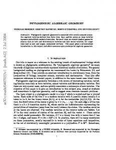
Theorem 2. Every function that can be obtained from a MAG to a given codomain set can also be obtained from a matrix representation of the MAG. Proof. Consider we show the commutative diagram depicted in Figure 5. In this figure, H is the set of all MAGs (up to isomorphism), J is the set of pairs of adjacency matrices and companion tuples (up to permutation), F is an arbitrary function from H to X, where X is a codomain consistent with the definition of function F, and I is the identity function in X. Since the function F is arbitrary, it can represent any function or algorithm, such as searches or centrality computations, which take MAGs to a result expected from this function. H

F

X I

ϒ J

Fˆ

X

Figure 5: Commutative diagram. As both functions ϒ (Equation (47) in Theorem 1) and I are isomorphisms, it follows that the depicted diagram commutes, so that for every function F : H Ñ X there is a function Fˆ : J Ñ X, which produces the same result. As a consequence of Theorem 2, it follows that, from the adjacency matrix and companion tuple of a MAG, one can obtain any possible outcome that can be obtained from a MAG or from any other representation equivalent to it, such as high order tensors, as those presented in recent related works [28, 46, 30]. Therefore, although we present a tensorial representation for MAGs, we do so only for the sake of completeness and will not use such representations for any algorithm.

4.3

Degree

The definition of degree in a traditional graph stems from the number of edges incident to a given vertex. This concept is generalized for MAGs in [32], where degrees can be defined for composite vertices, sub-determinations, or elements of a given aspect. Sub-determinations are defined as the cartesian product of a (proper) subset of the aspects of a given MAG. Further, since MAG edges are 37

considered to be directed, the degrees are also divided into out-degree and indegree. In this section, we present algorithms for calculating these distinct degree definitions. 4.3.1

Degree of composite vertices

The degree of composite vertices of a given MAG H is the degree of the vertices of the composite vertices representation of the MAG. Since the composite vertices representation, gpHq, is a traditional directed graph isomorphic to the MAG H, it follows that the degree determination is done with the traditional algorithm for directed graphs with minor changes. For a given MAG H and its companion tuple τpHq, the degrees of the composite vertices can be determined by Algorithm 8, where Dpπo peq, τpHqq and Dpπd peq, τpHqq stand for the numerical representation of the origin and destination composite vertices of edge e P EpHq, as defined in Section 3.2. input : H “ pA, Eq output: indegree, outdegrees Degree(H) 2 n Ð |VpHq| 3 T Ð CompTuplepApHqq // companion tuple of H, i.e. τpHq 4 indegree Ð vector of n integers, all 0 5 outdegree Ð vector of n integers, all 0 6 for each e P EpHq do 7 o Ð Dpπo peq, T q // numerical origin 8 d Ð Dpπd peq, T q // numerical destination 9 indegreerds Ð indegreerds ` 1 10 outdegreeros Ð outdegreeros ` 1 11 end 12 return indegree, outdegree Algorithm 8: Determination of the degree of composite vertices. 1

Another way for calculating the degress of the composite vertices is computing it algebraically from the adjacency matrix of the MAG, as given by indegree “ JpHqT 1, and 38

(50)

outdegree “ JpHq 1.

(51)

Further, the total degree of the composite vertices can be obtained by summing up their indegrees and outdegrees. To determine the time complexity of Algorithm 8, we consider that lines 2, 4, and 5 have each time complexity Op|VpHq|q, the determination of the companion tuple at line 3 has complexity Oppq, where p is the number of aspects of the MAG, so that p ! |VpHq|. Finally, since the determination of the numerical representation of vertices has complexity Oppq, we have that the for loop initiated at line 6 has complexity Opp ˚ |EpHq|q, so that the time complexity of Algorithm 8 is Op|VpHq| ` p ˚ |EpHq|q. If we consider that in a given case the order of the MAG does not vary, so that p is a constant, then the algorithm’s time complexity is Op|VpHq| ` |EpHq|q. In the case of the example MAG T (Figure 3), whose companion tuple is τ “ p3, 2, 3q, it can be seen that the composite vertex p2, Bus,t1q has outdegree 3 and indegree 1, while the composite vertex p1, Subway,t2q has outdegree 2 and indegree 2. Since Dpp2, Bus,t1q, τq “ 2 and Dpp1, Subway,t2q, τq “ 10, it follows that indegreer2s “ 1, outdegreer2s “ 3, indegreer10s “ 2 and outdegreer10s “ 2. 4.3.2

Degree of sub-determined vertices

We can determine the degree for sub-determined composite vertices in a similar way to the degree of composite vertices. Given a MAG H and a sub-determination ζ , the degree of the sub-determined composite vertices can be obtained by Algorithm 9, where |Vζ pHq| is the number of ζ sub-determined composite vertices on MAG H, Sζ is the function that takes a composite vertex to its subdetermined form, and Dζ is the function that takes the sub-determined composite vertex to its numerical representation. It can be seen that the time complexity of Algorithm 9 is the same as the time complexity of Algorithm 8. It is important to note that two distinct composite vertices may have the same sub-determined form. This happens when the two composite vertices differ only on aspects which are dropped by the sub-determination. In this case, the degree of each of these composite vertices is summed for obtain the sub-determined degree. From this, it can also be seen that some edges in the sub-determined form may become self-loops. The degrees calculated by Algorithm 9 include the self-loop edges. This algorithm can be modified to count the self-loops separately, as shown in Algorithm 10. This algorithm is similar to Algorithm 8 and has the same time complexity. 39

input : H “ pA, Eq, and ζ output: indegree, outdegree 1 2 3 4 5 6 7 8 9 10 11 12 13

SubDetDegree(H, ζ ) n Ð |Vζ pHq| T Ð CompTuplepApHqq // companion tuple of H, i.e. τpHq Tζ Ð τζ pHq // ζ sub-determined companion tuple indegree Ð vector of n integers, all 0 outdegree Ð vector of n integers, all 0 for each e P EpHq do o Ð Dpπo peq, Tζ q // numerical sub-determined origin d Ð Dpπd peq, Tζ q // numerical sub-determined destination indegreerds Ð indegreerds ` 1 outdegreeros Ð outdegreeros ` 1 end return indegree, outdegree Algorithm 9: Sub-determined degree.

The sub-determined composite vertices degree can also be determined algebraically with indegree “ Mζ pHq JpHqT 1,

(52)

outdegree “ Mζ pHq JpHq 1,

(53)

and

where Mζ pHq is the sub-determination matrix and 1 is the all 1s column vector, both defined in Section 4.1. Note that the multiplication by Mζ pHq adds the degrees of the composite vertices that are collapsed to the same sub-determined vertex. The degrees calculated by Equations (52) and (53) include the self-loop edges. To obtain the separate self-loop degrees, first note that Mζ pHq JpHq 1n “ Mζ pHq JpHq Mζ pHqT 1m .

(54)

This follows from the fact that Mζ pHqT 1m “ 1n , 40

(55)

input : H “ pA, Eq, and ζ output: indegree, sindegree, outdegree, soutdegree SubDetDegreeSepLoops(H, ζ ) 2 n Ð |Vζ pHq| 3 T Ð CompTuplepApHqq // companion tuple of H, i.e. τpHq 4 Tζ Ð τζ pHq // ζ sub-determined companion tuple 5 indegree Ð vector of n integers, all 0 6 outdegree Ð vector of n integers, all 0 7 sindegree Ð vector of n integers, all 0 8 soutdegree Ð vector of n integers, all 0 9 for each e P EpHq do 10 o Ð Dpπo peq, Tζ q // numerical sub-determined origin 11 d Ð Dpπd peq, Tζ q // numerical sub-determined destination 12 if d ‰ o then 13 indegreerds Ð indegreerds ` 1 14 outdegreeros Ð outdegreeros ` 1 15 end 16 else 17 sindegreerds Ð sindegreerds ` 1 18 soutdegreeros Ð soutdegreeros ` 1 19 end 20 end 21 return indegree, sindegree, outdegree, soutdegree Algorithm 10: Sub-determined degree, separating self-loops 1

since Mζ pHqT is a n ˆ m rectangular matrix and has the property that each row has exactly one non-zero entry of value 1. Furthermore, note that the matrix Mζ pHq JpHq Mζ pHqT is the adjacency matrix of the sub-determined MAG Hζ . Since the composite vertices representation of a sub-determined MAG is a multigraph, each non-zero entry shows the number of superposed edges in the sub-determination. Therefore, the main diagonal of Mζ pHq JpHq Mζ pHqT has the self-loop degree of each vertex. Hence, sindegree “ DiagpMζ pHq JpHqT Mζ pHqT q,

(56)

soutdegree “ DiagpMζ pHq JpHq Mζ pHqT q.

(57)

and

41

For example, consider the example MAG T (Figure 3) and the sub-determination ζt “ p1, 1, 0q defined in Section 4.1. We have that » fi 0 7 4 4 7 0

— — T indegree “ Mζ t pT q JpT q 1 “ — — – »

0 7 4 4 7 0

— — outdegree “ Mζ t pT q JpT q 1 “ — — – » — — Mζ t pT q JpT q Mζ t pT q “ — — – T

0 0 0 0 0 0

0 2 2 0 3 0

and

0 2 2 0 0 0

0 0 0 2 2 0

» — — DiagpMζ t pT q JpT q Mζ t pT q q “ — — – T

ffi ffi ffi , ffi fl fi ffi ffi ffi , ffi fl 0 3 0 2 2 0

0 2 2 2 2 0

(58)

(59)

0 0 0 0 0 0

fi ffi ffi ffi , ffi fl

(60)

fi ffi ffi ffi . ffi fl

(61)

This means that, for instance, the sub-determined composite vertex p2, Subwayq has outdegree 7, indegree 7, and 2 self-loops. This sub-determination corresponds to the aggregation of all 3 time instants, which means that the edges in which only the time instant changes become self-loops. These edges are shown in red (dotted) in Figure 3. Note that τζt “ p2, 3q, so that Dpp2, Subwayq, p2, 3qq “ 2, making it correspond to the second element of the degree column vector. 4.3.3

Single aspect degree

The single aspect degree is a particular case of sub-determined degree in which the sub-determination applied is such that only a single aspect remains. Therefore, the determination of single aspect degrees is done in the same way presented in Section 4.3.2. 42

We, however, present an additional example illustrating the time instant degree, which is obtained by the sub-determination ζT “ p0, 0, 1q defined in Section 4.1. This sub-determination has only the third aspect of the MAG T (Figure 3), which corresponds to the three time instants present on MAG T . In this case, we have that « ff 2 10 10

indegree “ Mζ T pT q JpT qT 1 “ « outdegree “ Mζ T pT q JpT q 1 “ « Mζ T pT q JpT q Mζ T pT qT “

2 0 0

,

(63)

ff

0 8 2

ff

2 2 2

ff

« DiagpMζ T pT q JpT q Mζ T pT qT q “

(62)

10 10 2

8 2 0

and

,

,

.

(64)

(65)

Therefore, we have that τζT “ p3q, so that Dppt1 q, p3qq “ 1, Dppt2 q, p3qq “ 2, and Dppt3 q, p3qq “ 3. Considering the composite vertices representation of MAG T , depicted in Figure 3, it can be seen that each time instant has 2 self-loop edges (in blue-dashed), which is consistent with Equation (65). Further, there are 8 edges from t1 to t2 (in red-dotted and black) and 8 edges from t2 to t3 . This is consistent with the adjacency matrix shown in Equation (64). Further, the indegrees and outdegrees of each time instant are consistent with Equations (62) and (63).

4.4

Breadth-First Search (BFS)

The Breadth-First Search (BFS) is an important graph algorithm that can be seen as a primitive for building many other algorithms [7]. The goal of this subsection is to illustrate how the BFS algorithm can be adapted for being used in MAGs, both in its full composite vertices representation and in its sub-determined forms. In the not sub-determined form, the adaptation is very simple, since the composite vertices representation of a MAG is a directed graph. In this case, all that is needed is to convert the composite vertices representation from its tuple to numerical form, and then apply the traditional BFS algorithm. The adaptation to the subdetermined forms also does not require major changes on the algorithm. As with 43

many graph algorithms, BFS can be expressed in combinational or in algebraic forms, which are presented in the following related sub-sections. 4.4.1

BFS for composite vertices

The non sub-determined BFS in its combinational form is constructed directly upon the MAG’s adjacency matrix, JpHq. In particular, the form presented in Algorithm 11 gets the neighbors of a given composite vertex s from the row corresponding to it in the adjacency matrix. Note that the row of a given composite vertex has 1s in the columns that correspond to the neighbors of the given vertex. Therefore, the expression “each v P JpHqru, ¨s” in line 12 of Algorithm 11 means “the number of each column for which there is a 1 at row u”. In this case, we consider that JpHq is a CSR sparse matrix [41], in which the operation of extracting the non-zero entries of a row is straightforward and efficient. Considering Algorithm 11 and the standard form of the BFS algorithm encountered in [7], it can be seen that the difference is that each composite vertex has to be transformed from its tuple representation to its numerical representation, as shown in lines 8,9 and 10 of Algorithm 11. Therefore, from the analysis provided in [7], we can conclude that the time complexity of Algorithm 11 is Op|VpHq| ` |EpHq|q. BFS is also closely related to matrix multiplication. This stems from the wellknown property of the powers of the adjacency matrix, in which the pi, jq entry of the n-th power of the adjacency matrix shows the number of existing walks of length n from vertex i to vertex j [41]. From this, we could think that for a given MAG H, the series B“

8 ÿ

JpHqi “ I ` JpHq ` JpHq2 ` JpHq3 ` JpHq4 ` . . .

(66)

i“0

would produce a matrix B, such that the entry Bi, j indicates the number of walks of any length from vertex i to vertex j. This is indeed the case when H happens to be an acyclic MAG, making JpHq a nilpotent matrix. The existence of cycles in H makes that, for some vertices, there will exist walks of arbitrary length connecting them (namely, the cycles), making the series of Equation (66) divergent. However, since the objective is not to know the number of walks between each pair of vertices, but simply to know which vertices are reachable from each other (i.e. there is at least a path between them), this technical problem can be solved by multiplying the adjacency matrix JpHq by a scalar 44

input : JpHq, τpHq, and s P VpHq output: vertices, distance, pred 1 2 3 4 5 6 7 8 9 10 11 12 13 14 15 16 17 18 19 20 21 22 23 24 25

BFS(JpHq, τpHq, s) n Ð |VpHq| vertices Ð vector of n integers, all 0 distance Ð vector of n integers, all 8 pred Ð vector of n integers, all Nil color Ð vector of n integers, all 0 Q Ð empty queue verticesrDps, Tauq ´ 1s Ð 1 distancerDps, τpHqqs Ð 0 EnqueuepQ, Dps, τpHqqq while Q not empty do u Ð headrQs for each v P JpHqru, ¨s do if colorrvs “ 0 then colorrvs Ð 1 verticesrvs Ð 1 distancervs Ð distancerus ` 1 predrvs Ð u EnqueuepQ, vq end end DequeuepQq colorrus Ð 2 end return vertices, distance, pred Algorithm 11: BFS for composite vertices.

ρH , such that ρH ă

1 , ρpJpHqq

(67)

where ρpJpHqq is the spectral radius of the matrix JpHq. This leads to the matrix Jρ pHq “ ρH JpHq,

(68)

so that the spectral radius of the matrix Jρ pHq ă 1 and this results that Equa45

tion (66) constructed with the matrix Jρ pHq converges. Since the convergence of the series is assured, Equation (66) can be re-expressed as B “ pI ´ Jρ pHqq´1 .

(69)

The matrix B defined in Equation (69) has the property that, for any given composite vertex v P VpHq, the row Dpvq of B has non-zero entries in every column that corresponds to a composite vertex u P VpHq, such that u is reachable from v. Hence, for a given composite vertex v, the row Dpvq corresponds to the result of a BFS started at that composite vertex. Although the matrix B carries the BFS of all composite vertices of the MAG H, it is important to note that this matrix may not be sparse, which for large MAGs can lead to difficulties in memory allocation. In order to avoid such difficulties, it is also possible to express a BFS for a single composite vertex v as B “ rv I ` rv Jρ pHq ` rv Jρ pHq2 ` rv Jρ pHq3 ` rv Jρ pHq4 ` . . . ,

(70)

where rv is the row vector with n entries for which all entries except Dpv, τq are 0 and the entry Dpv, τq is 1. Considering the example MAG T , shown in Figure 3, the result of the BFS using Algorithm 11 for the composite vertex p2, Bus,t1 q, whose numerical representation is Dpp2, Bus,t1 q, p3, 2, 3qq “ 2, is vertices “ r2, 5, 8, 9, 10, 11, 14, 15, 16, 17s (71) distances “ r8, 0, 8, 8, 1, 8, 8, 1, 1, 2, 2, 8, 8, 2, 2, 3, 3, 8s pred “ rNil, Nil, Nil, Nil, 2, Nil, Nil, 2, 2, 5, 5, Nil, Nil, 8, 8, 10, 10, Nils,

where the list vertices shows the composite vertices accessible from p2, Bus,t1 q, which in this example represent all locations, transportation modals, and time instants reachable from this initial point. The list distances carries the distances in hops from the initial composite vertex p2, Bus,t1 q to all possible destinations (with 8 meaning that a destination is not reachable). The list pred shows the predecessors of each composite vertex, making possible to construct a BFS tree. 4.4.2

Sub-determined BFS

It is possible to obtain a sub-determined form of the BFS algorithm for MAGs. It is important, however, to realize that this sub-determined BFS algorithm is not 46

(a) MAG R

(b) Sub-determined form

Figure 6: MAG R and its sub-determined form. equivalent to applying the BFS algorithms presented in Section 4.4.1 to a subdetermined MAG. A sub-determination is a generalization of the idea of aggregating multilayer and time-varying graphs, as shown in Section 2.2. As with the aggregation process, the sub-determination of a MAG can cause the presence of paths and walks on the sub-determined MAG that do not actually exist on the original form. To illustrate this, we present Figures 6a and 6b, which show a small two aspects MAG and its sub-determined form, obtained by the sub-determination ζR “ p1, 0q. First, note that, in the MAG R shown in Figure 6a, there is no path originating from the composite vertices p1, 1q or p1, 2q to the composite vertices p3, 1q or p3, 2q. Nevertheless, in Figure 6b, there is a path connecting the subdetermined vertex p1q to the sub-determined vertex p3q, even though such connection is not possible on the original MAG shown in Figure 6a. Therefore, in order to obtain the proper result, the sub-determined BFS can not be evaluated directly using the sub-determined MAG. Such a case can be seen algebraically by noting that given a MAG H and a sub-determination ζ , in general ˜ ¸ 8 8 ÿ ÿ ` ˘i T i Mζ pHq Jρ pHq Mζ pHq ‰ Mζ pHq Jρ pHq Mζ pHqT . (72) i“0

i“0

To see that the Inequality (72) holds, note that an arbitrary power of the matrix

47

Mζ pHq Jρ pHq Mζ pHqT is given by `

Mζ pHqJρ pHqMζ pHqT

˘n

T T “M ζ pHqJρ pHqMζ pHq Mζ pHqJρ pHqMζ pHq . . ., loooooooooooooooooooooooooooooomoooooooooooooooooooooooooooooon n times

(73) ` ˘ where Mζ pHq Jρ pHq Mζ pHqT is multiplied n times. Note, however, that Mζ pHqT Mζ pHq ‰ In ,

(74)

since Mζ pHq P Rmˆn is a retangular matrix and m ă n, so that the rank of the matrix Mζ pHqT Mζ pHq is less or equal to m, while the rank of the identity In is n ą m. Since Inequality (74) holds, so does the Inequality (72). Here, the left hand side of the Inequality (72) corresponds to the sub-determination of the BFS calculated for the MAG H, while the right hand side corresponds to the BFS calculated for the sub-determined MAG Hζ . In the case of the MAG R, shown in Figure 6a, we have that the sub-determination is given by ζR “ p1, 0q and the adjacency and sub-determination matrices are fi » — — JpRq “ — — –

0 0 0 1 0 0 0 1 0 1 0 0 0 0 0 0 0 0 0 1 0 0 0 0 0 0 0 0 0 0

« MζR pRq “

1 0 0

and

0 1 0

« JζR pRq “

0 0 0

0 0 1 0 0 0

1 0 0

0 1 0

1 0 0 1 0 0

ff

0 0 1

ffi ffi ffi , ffi fl

(75)

ff

0 0 1

,

(76)

.

(77)

Therefore, we have that ˜ MζR pRq

8 ÿ

¸ Jρ pRqi

« MζR pRqT “

i“0

while

8 ÿ `

« MζR pRq Jρ pRq MζR pRq

i“0

48

˘ T i

“

3 0 0

2 3 0

0 2 3

ff

2 0 0

2 2 0

2 2 2

ff

,

(78)

(79)

and

« `

I3 ´ JζR pRq

˘´1

“

1 0 0

1 1 0

1 1 1

ff .

(80)

Remembering that the entries of the matrices in Equations (78), (79), and (80) are to be considered only as zero or non-zero, it can be seen that the matrix at Equation (78) has a 0 at entry p1, 3q, while the matrices at Equations (79) and (80) have a non-zero entry at this same position. This illustrates the situation in which a BFS is done on the sub-determined (aggregated) MAG, as in Equations (79) and (80), i.e. paths that are not present on the original MAG can appear on the sub-determined form, potentially altering the results obtained by algorithms applied to it. For instance, considering the MAG T , depicted in Figure 3, for a sub-determination ζt “ p1, 1, 0q, which drops the time aspect, and considering ρH “ 0.5 so that Jρ pT q “ 0.5 JpT q, we have that fi » ˜ Mζ t pT q

8 ÿ

i“0

¸ i

Jρ pT q

— — T Mζ t pT q “ — — –

3 0 0 0 0 0 7.8 2.2 1.3 5.2 0 2.2 4.6 0.2 1.3 0 1.3 0.2 4.6 2.2 0 5.2 1.3 2.2 7.8 0 0 0 0 0

0 0 0 0 0 3

ffi ffi ffi . ffi fl

(81)

Algorithm 12 shows a combinational version of the sub-determined BFS. As previously stated, this algorithm evaluates the BFS on the MAG without subdetermination and after that sub-determines the obtained results. This procedure ensures that only paths present on the original MAG are considered on the subdetermined BFS. The sub-determination of the results obtained from the BFS is done in the internal if, comprising lines 21 to 25 of Algorithm 12. After applying Algorithm 12 to the MAG R with initial vertex s “ 1 and subdetemination ζR “ p1, 0q, the obtained result is vertices “ r1, 2s distances “ r0, 1, 8s pred “ rNil, 1, Nils,

(82)

which is consistent with the result obtained by Equation (78). Further, applying Algorithm 12 to MAG T , shown in Figure 3, with starting composite vertex s “ p2, Busq and applying the sub-determination ζt “ p1, 1, 0q, 49

1 2 3 4 5 6 7 8 9 10 11 12 13 14 15 16 17 18 19 20 21 22 23 24 25 26 27 28 29 30 31 32 33

input : JpHq, τpHq, ζ and s P Vζ pHq output: vertices, distance, pred BFS-Sub(JpHq, τpHq, ζ , s) n Ð |VpHq| nS Ð |Vζ pHq| Tζ Ð τζ pHq // ζ sub-determined companion tuple vertices Ð vector of nS integers, all 0 distance Ð vector of nS integers, all 8 pred Ð vector of nS integers, all Nil colorS Ð vector of nS integers, all 0 color Ð vector of n integers, all 0 Q Ð empty queue for every v P VpHq where Dpv, τζ pHqq “ Dps, τζ pHqq do EnqueuepQ, Dpv, τpHqqq colorrDpv, τpHqqs Ð 1 end verticesrDps, T zq ´ 1s Ð 1 distancerDps, Tζ qs Ð 0 while Q not empty do u Ð headrQs for each v P JpHqru, ¨s do if colorrvs “ 0 then colorrvs Ð 1 EnqueuepQ, vq if colorSrDpv, Tζ qs “ 0 then colorSrDpv, Tζ qs Ð 1 verticesrDpv, Tζ qs Ð 1 distancerDpv, Tζ qs Ð distancerDpu, Tζ qs ` 1 predrDpv, Tζ qs Ð Dpu, Tζ q end end end colorrus Ð 2 DequeuepQq end return vertices, distance, pred

Algorithm 12: Sub-determined BFS.

50

which drops the time aspect, the obtained result is vertices “ r2, 5, 3, 4s distances “ r8, 0, 1, 2, 1, 8s pred “ rNil, Nil, 2, 5, 2, Nils.

(83)

Considering that τζt “ p3, 2q and 2 “ Dpp2, Busq, p3, 2qq, 5 “ Dpp2, Subwayq, p3, 2qq, 3 “ Dpp3, Busq, p3, 2qq, and 1 “ Dpp1, Subwayq, p3, 2qq, this means that disregarding time, starting from p2, Busq it is possible to reach p2, Subwayq in 1 step, p1, Subwayq in 2 steps, and p3, Busq in 1 step. It is not possible to reach p1, Busq because there is no bus stop at location 1, neither p3, Subwayq because there is no subway station at location 3. From the predecessor list (pred) it is possible to build a BFS tree, where p2, Busq is the root, p2, Subwayq and p3, Busq are children of p2, Busq, and p1, Subwayq is a child of p2, Subwayq. Note that p1, Subwayq and p3, Busq are leaves. It can be seen that the result obtained in Equation (81) is consistent with the results obtained by Algorithm 12. Comparing Algorithm 12 to Algorithm 11, it can be seen that the main difference is the additional for loop at line 12 of Algorithm 12. Since the time complexity of this loop is Op|VpHq|q, we then conclude that the time complexity of Algorithm 12 is Op|VpHq| ` |EpHq|q. 4.4.3

Single aspect BFS

The single aspect BFS is a special case of the sub-determined BFS. As such, it is evaluated using the same algorithms presented in Section 4.4.2 for the subdetermined case. Considering the example MAG T (Figure 3), a sub-determination ζL “ p1, 0, 0q, which drops the time and transportation mode aspects (thus leaving only the locations aspect), and making ρH “ 0.5 so that Jρ pT q “ 0.5 JpT q, we have that ˜ ¸ « ff 8 7.6 3.5 0.2 ÿ i T MζL pT q Jρ pT q MζL pT q “ 3.5 26 3.5 , (84) 0.2

i“0

3.5

7.6

indicating that disregarding the aspects of time instants and transportation modes, all locations can be reached from any location. Applying Algorithm 12 to the MAG T , with starting composite vertex s “ p1q and employing the sub-determination ζL “ p1, 0, 0q, which drops the aspects of

51

the transportation mode and time instants, the obtained result is vertices “ r1, 2, 3s distances “ r0, 1, 2s pred “ rNil, 1, 2s,

(85)

which is consistent with the result obtained by Equation (84).

4.5

Depth-First Search (DFS)

In this section, we show the adaptation of the Depth-First Search (DFS) algorithm for use with MAGs. The DFS algorithm exposes many properties of the MAG structure and is used as a primitive for the construction of many other algorithms [7]. We present DFS algorithms for both the full composite vertices representation of the MAG as well as for the sub-determined form. We remark that in the sub-determined algorithm the full information of the MAG is used, in the sense of preventing the use of paths that may exist in the sub-determined form of the MAG, while not actually existing in the original MAG. 4.5.1

DFS for composite vertices

The composite vertices implementation is constructed using the MAG’s adjacency matrix JpHq and companion tuple τpHq. The implementation shown is very similar to the traditional implementation presented in [7], which is expected since the composite vertices representation of the MAG is indeed a directed graph, so that the original algorithm applies. The proposed implementation can be seen in Algorithm 13, which is similar to the original implementation, except for the use of a sparse matrix as the representation of the MAG. This leads to the expression “each v P JpHqru, ¨s at line 5 of Procedure DFS-Visit, which should be read as “the number of each column for which there is a 1 at row u”. Since JpHq is a CSR sparse matrix [41], the operation of extracting the non-zero entries of a row is straightforward and efficient. Considering the analysis provided in [7], we conclude that the time complexity of Algorithm 13 is Op|VpHq| ` |EpHq|q. When applied to MAG T , shown in Fig-

52

ure 3, the DFS algorithm generates the result d “ r0, 2, 22, 24, 3, 26, 28, 13, 19, 4, 12, 30, 32, 8, 14, 5, 7, 34s (86) f “ r1, 21, 23, 25, 18, 27, 29, 16, 20, 11, 17, 31, 33, 9, 15, 6, 10, 35s pred “ rNil, Nil, Nil, Nil, 2, Nil, Nil, 11, 2, 5, 5, Nil, Nil, 17, 8, 10, 10, Nils,

where the list d carries the discovery time of each composite vertex, the list f the respective finish time of each composite vertex, and pred the predecessor list of each composite vertex. 4.5.2

Sub-determined DFS

The sub-determined DFS algorithm is presented in Algorithm 14 and is similar to the non sub-determined one. The main differences are at the Procedure Visit-DFSSub and the call to a sub-determined BFS at line 15 of the DFS-Sub function. This version for a sub-determined BFS is considered in order to determine reachability of sub-determined vertices from the root of each sub-determined DFS tree. This is necessary to prevent including vertices not reachable from the tree root in the non sub-determined MAG into the DFS trees constructed by Procedure Visit-DFSSub. An example of this is provided in Equation (88). The difference in Procedure Visit-DFS-Sub is that in addition to the root vertex for the DFS tree it also receives the reachability vector produced by the BFS. This reachability vector has one entry for each sub-determined vertex. This entry has value 1 when corresponding to a reachable vertex, while entries corresponding to unreachable vertices carry value 0. In order to determine the time complexity of Algorithm 14, we consider that the sub-determined BFS executed at line 15 of Function DFS-Sub is done once for the root node of each sub-determined DFS tree. Since it is executed only once for each DFS tree, we conclude that the total time expended in the subdetermined BFS algorithm is Op|VpHq| ` |EpHq|q. Since the reachability check included in Function Visit-DFS-Sub is done by verifying the content of one entry of the reachability vector, it is done in Op1q and therefore does not affect the overall time complexity of the Visit-DFS-Sub Function. Therefore, since the DFS is run upon the sub-determined MAG, it follows that the time complexity of doing the DFS part of the Algorithm is Op|Vζ pHq| ` |Eζ pHq|q. Since |Vζ pHq| ă |VpHq| and |Eζ pHq| ă |EpHq|, we conclude that the time complexity is dominated by the

53

input : JpHq, τpHq output: discTime, f inTime, pred 1 2 3 4 5 6 7 8 9 10 11 12 13 14 15 1 2 3 4 5 6 7 8 9 10 11 12 13

DFS(JpHq, τpHq) n Ð |VpHq| for u “ 1 to n do colorrus Ð 0 discTimerus Ð ´1 f inTimerus Ð ´1 predrus Ð ´1 end time Ð 0 for u “ 1 to n do if colorrus “ 0 then DFS-Visitpuq end end return discTime, f inTime, pred

// set all vertices to white // set discovery times to nil // set finish times to nil // set predecessors to nil

Procedure DFS-Visit(u) colorrus Ð 1 // set vertex u to gray discTimerus Ð time time Ð time ` 1 for each v P JpHqru, ¨s do if colorrvs “ 0 then predrvs Ð u DFS-Visitpvq end end colorrus Ð 2 // set vertex u to black f inTimerus Ð time time Ð time ` 1 Algorithm 13: DFS for composite vertices.

BFS used for the reachability determination, making the overall time complexity of Algorithm 14 to be Op|VpHq| ` |EpHq|q. When applying the sub-determined DFS algorithm to the example MAG T

54

1 2 3 4 5 6 7 8 9 10 11 12 13 14 15 16 17 18 19 1 2 3 4 5 6 7 8 9 10 11 12 13

input : JpHq, τpHq,ζ output: discTime, f inTime, pred DFS-Sub(JpHq, τpHq,ζ ) Tζ Ð τζ pHq // ζ sub-determined companion tuple Mζ Ð SubDetMatrixpH, ζ q Jζ “ Mζ JpHq MTζ // Sub-determined adjacency matrix n Ð |Vζ pHq| // number of sub-determined vertices for u “ 1 to n do colorrus Ð 0 // set all vertices to white discTimerus Ð ´1 // set discovery times to nil f inTimerus Ð ´1 // set finish times to nil predrus Ð ´1 // set predecessors to nil end time Ð 0 for u “ 1 to n do if colorrus “ 0 then vertices “ BFS-SubpJpHq, τpHq, ζ , Tζ q DFS-Visit-Subpu, verticesq end end return discTime, f inTime, pred Procedure DFS-Visit-Sub(u, vertices) colorrus Ð 1 // set vertex u to gray discTimerus Ð time time Ð time ` 1 for each v P Jζ ru, ¨s do if colorrvs “ 0 and verticesrvs ‰ 0 then predrvs Ð u DFS-Visit-Subpv, verticesq end end colorrus Ð 2 // set vertex u to black f inTimerus Ð time time Ð time ` 1

Algorithm 14: Sub-determined DFS. shown in Figure 3 with a sub-determination ζt “ p1, 1, 0q, which drops the time

55

aspect, the obtained result is d “ r0, 2, 3, 6, 5, 10s f “ r1, 9, 4, 7, 8, 11s pred “ rNil, Nil, 2, 5, 2, Nils,

(87)

where the list d carries the discovery time of each sub-determined composite vertex, the list f its finish time and pred its predecessor. Considering the MAG R shown in Figure 6a with a sub-determination ζR “ p1, 0q, the result obtained by Algorithm 14 is d “ r0, 1, 4s f “ r3, 2, 5s pred “ rNil, 1, Nils.

(88)

It can be seen that even though in the MAG R sub-determined by ζR “ p1, 0q (see Figure 6b) there is a path from vertex 1 to 3, vertex 3 is not in the same DFS tree as vertices 1 and 2, even with the DFS starting at vertex 1, as can be seen in dr0s. This occurs because in MAG R (with no sub-determination) there is no path connecting the composite vertex 1 to the composite vertex 3. 4.5.3

Single aspect DFS

The single aspect DFS is a special case of the sub-determined DFS. As such, it is evaluated using the same algorithms presented for the sub-determined case in Section 4.5.2. Applying Algorithm 14 to MAG T (Figure 3), and employing the sub-determination ζL “ p1, 0, 0q, which drops the aspects of transportation modes and time instants, the obtained result is d “ r0, 1, 2s f “ r5, 4, 3s pred “ rNil, 1, 2s,

(89)

where the list d carries the discovery time of each sub-determined composite vertex, the list f its finish time, and pred its predecessor. 56

5

Final remarks

In this paper, we have presented the algebraic representation and basic algorithms of MultiAspect Graphs (MAGs). The key contribution has been to show that models based on the MAG abstraction (formally defined in [32]) can be represented by a matrix and a companion tuple. Furthermore, we have also shown that any possible MAG function (algorithm) can be obtained from this matrix-based representation. This is an important theoretical result because it paves the way for adapting well-known graph algorithms for application in MAGs. In this sense, we have presented the adaptation for the MAG context of basic graph algorithms, such as computing degree, BFS, and DFS. In particular, we have also presented the sub-determined versions of the same basic algorithms, showing that such versions disregard spurious paths that usually result from the sub-determination process, thus avoiding the pollution of the results with the consideration of such paths. As future work, we intend to build upon the results here obtained for the algebraic representation and basic algorithms of MAGs to analyze MAG properties, such as the centrality of edges, composite vertices, and aspects. We also intend to consider the dynamics encountered in these properties in the cases where one of the MAG aspects represents time. Finally, we are also targeting the application of the MAG concept for the better understanding, modeling, and analysis of different complex networked systems found in real-world applications.

Acknowledgment This work was partially funded by the Brazilian funding agencies CAPES, CNPq, FINEP, and FAPERJ as well as the Brazilian Ministry of Science, Technology, and Innovation (MCTI).

References [1] P. Erd¨os, A. R´enyi, On random graphs I, Publicationes Mathematicae (Debrecen) 6 (1959) 290–297. [2] P. Erd¨os, A. R´enyi, On the evolution of random graphs, Publication of the Mathematical Institute of the Hungarian Academy of Sciences, (1960) 17– 61.

57

[3] R. Tarjan, Depth-First Search and Linear Graph Algorithms, SIAM Journal on Computing, 1 (2) (1972) 146–160. [4] M. Fiedler, Algebraic Connectivity of Graphs, Czechoslovak Mathematical Journal, 23 (2) (1973) 298–305. [5] B. Mohar, The Laplacian spectrum of graphs, in: Y. Alavi, G. Chartrand, O. R. Oellermann, A. J. Schwenk (Eds.), Graph Theory, Combinatorics, and Applications, Wiley, (1991) 871–898. [6] L. Lov´asz, Random walks on graphs: A survey, Combinatorics, Paul Erd¨os is eighty, (Volume 2) (1993) 1–46. [7] T. H. Cormen, C. Stein, R. L. Rivest, C. E. Leiserson, Introduction to Algorithms, 2nd Edition, McGraw-Hill Higher Education, (2001). [8] L. Freeman, Centrality in social networks conceptual clarification, Social Networks, 1 (3) (1979) 215–239. [9] P. Bonacich, Power and centrality: A family of measures, The American Journal of Sociology, 92 (5) (1987) 1170–1182. [10] N. Friedkin, Theoretical foundations for centrality measures, The American Journal of Sociology, 96 (6) (1991) 1478–1504. [11] P. Bonacich, Some unique properties of eigenvector centrality, Social Networks, 29 (4) (2007) 555–564. [12] D. Watts, S. H. Strogatz, Collective dynamics of small-world networks, Nature, 393 (June) (1998) 440–442. [13] A. Barab´asi, R. Albert, Emergence of Scaling in Random Networks, Science, 286 (5439) (1999) 509–512. [14] R. Albert, H. Jeong, A. Barabasi, Error and attack tolerance of complex networks, Nature, 406 (6794) (2000) 378–82. [15] R. Pastor-Satorras, A. Vespignani, Epidemic spreading in scale-free networks, Physical Review Letters, 86 (14) (2001) 3200–3203.

58

´ Tardos Maximizing the Spread of Influence [16] D. Kempe, J. Kleinberg, E. through a Social Network, Proceedings of the ninth ACM SIGKDD international conference on Knowledge discovery and data mining - KDD ’03, (2003) 137–146. [17] M. Kurant, P. Thiran, Layered Complex Networks, Physical Review Letters, 96 (13) (2006) 138701. [18] S. V. Buldyrev, R. Parshani, G. Paul, H. E. Stanley, S. Havlin, Catastrophic cascade of failures in interdependent networks., Nature, 464 (7291) (2010) 1025–8. [19] M. Szell, R. Lambiotte, S. Thurner, Multirelational organization of largescale social networks in an online world., Proceedings of the National Academy of Sciences of the United States of America, 107 (31) (2010) 13636–41. [20] D. Kempe, J. Kleinberg, A. Kumar, Connectivity and Inference Problems for Temporal Networks, Journal of Computer and System Sciences, 64 (4) (2002) 820–842. [21] A. Ferreira, On models and algorithms for dynamic communication networks: The case for evolving graphs, Proceedings of ALGOTEL Quatri`emes Rencontres Francophones sur les aspects Algorithmiques des T´el´ecommunications, (2002). [22] J. Leskovec, J. Kleinberg, C. Faloutsos, Graphs over time, in: Proc. of the ACM Int. Conference on Knowledge Discovery in Data Mining (KDD), ACM Press, New York, New York, USA, (2005) 177–187. [23] V. Kostakos, Temporal graphs, Physica A: Statistical Mechanics and its Applications, 388 (6) (2009) 1007–1023. [24] J. Tang, S. Scellato, M. Musolesi, C. Mascolo, V. Latora, Small-world behavior in time-varying graphs, Physical Review E, 81 (5) (2010) 81–84. [25] A. Casteigts, P. Flocchini, W. Quattrociocchi, N. Santoro, Time-varying graphs and dynamic networks, International Journal of Parallel, Emergent and Distributed Systems, 27 (5) (2012) 387–408.

59

[26] H. Kim, R. Anderson, Temporal node centrality in complex networks, Physical Review E, 85 (2) (2012). [27] K. Wehmuth, A. Ziviani, E. Fleury, A Unifying Model for Representing Time-Varying Graphs, Technical Report RR-8466, INRIA (2014). URL http://hal.inria.fr/hal-00941622 [28] M. De Domenico, A. Sol´e-Ribalta, E. Cozzo, M. Kivel¨a, Y. Moreno, M. Porter, S. G´omez, A. Arenas, Mathematical Formulation of Multilayer Networks, Physical Review X, 3 (4) (2013) 041022. [29] M. De Domenico, A. Sole, S. Gomez, A. Arenas, Random Walks on Multiplex Networks, arXiv, (2013) arXiv:1306.0519. [30] M. Kivel¨a, A. Arenas, M. Barthelemy, J. P. Gleeson, Y. Moreno, M. a. Porter, Multilayer Networks, Journal of Complex Networks, (2014). [31] S. Boccaletti, G. Bianconi, R. Criado, C. I. del Genio, J. G´omez-Garde˜nes, M. Romance, I. Sendi˜na Nadal, Z. Wang, M. Zanin, The structure and dynamics of multilayer networks, Physics Reports, 544 (1) (2014) 1–122. [32] K. Wehmuth, E. Fleury, A. Ziviani, On MultiAspect Graphs, arXiv, (2014) arXiv:1408.0943. [33] J. C. Lucet, C. Laouenan, G. Chelius, N. Veziris, D. Lepelletier, A. Friggeri, D. Abiteboul, E. Bouvet, F. Mentre, E. Fleury, Electronic Sensors for Assessing Interactions between Healthcare Workers and Patients under Airborne Precautions, PLoS ONE, 7 (5) (2012) e37893. [34] C. Sarraute, J. Brea, J. Burroni, K. Wehmuth, A. Ziviani, J. I. AlvarezHamelin, Social Events in a Time-Varying Mobile Phone Graph, in: Conference on the Scientific Analysis of Mobile Phone Datasets (NetMob 2015), Cambridge, MA, USA, (2015) 123–125. [35] G. Lulli, M. Romauch, A mathematical program to refine gene regulatory networks, Discrete Applied Mathematics, 157 (10) (2009) 2469–2482. [36] R. Z. Farahani, E. Miandoabchi, W. Y. Szeto, H. Rashidi, A review of urban transportation network design problems, European Journal of Operational Research, 229 (2) (2013) 281–302.

60

[37] E. Bullmore, O. Sporns, Complex brain networks: graph theoretical analysis of structural and functional systems., Nature reviews. Neuroscience, 10 (3) (2009) 186–98. [38] F. Chung, Lectures on spectral graph theory, CBMS Lectures, Fresno, (1996). [39] J. Bang-Jensen, G. Z. Gutin, Digraphs: Theory, Algorithms and Applications, 2nd Edition, Springer Publishing Company, Incorporated, (2008). [40] R. Distel, Graph Theory, 4th Edition, Springer Publishing Company, Incorporated, (2010). [41] J. Kepner, J. Gilbert, Graph Algorithms in the Language of Linear Algebra, SIAM, (2011). [42] L.-H. Lim, Singular Values and Eigenvalues of Tensors: A Variational Approach, in: 1st IEEE International Workshop on Computational Advances in Multi-Sensor Adaptive Processing, 2005., no. 1, IEEE, (2005) 129–132. [43] T. G. Kolda, Multilinear operators for higher-order decompositions, Tech. Rep. April, Sandia National Laboratories (2006). [44] R. B. Bapat, Graphs and Matrices, Springer, (2010). [45] A. Sol´e-Ribalta, M. De Domenico, N. E. Kouvaris, A. D´ıaz-Guilera, S. G´omez, A. Arenas, Spectral properties of the Laplacian of multiplex networks, Physical Review E, 88 (3) (2013) 032807. [46] M. De Domenico, A. Sol´e-Ribalta, E. Omodei, S. G´omez, A. Arenas, Centrality in Interconnected Multilayer Networks, arXiv, (2013) arXiv: 1311.2906.

61