grid transfer operators for highly variable coefficient ... - Cerfacs

GRID TRANSFER OPERATORS FOR HIGHLY VARIABLE COEFFICIENT PROBLEMS IN TWO-LEVEL NON-OVERLAPPING DOMAIN DECOMPOSITION METHODS L. GIRAUD∗ , F. GUEVARA VASQUEZ

∗ , AND

R. S. TUMINARO†

CERFACS Tech. Rep.: TR/PA/01/03 Abstract. We propose a robust interpolation scheme for non-overlapping two-level domain decomposition methods applied to two-dimensional elliptic problems with discontinuous coefficients. This interpolation is used to design a preconditioner closely related to the BPS scheme proposed in [1]. Through numerical experiments, we show on structured and unstructured finite element problems that the new preconditioning scheme reduces to the BPS method on smooth problems but outperforms it on problems with discontinuous coefficients. In particular it maintains good scalable convergence behavior even when the jumps in the coefficients are not aligned with subdomain interfaces. Keywords : Domain decomposition, two-level preconditioning, Schur complement, parallel distributed computing, elliptic partial differential equations, discontinuous coefficients.

1. Introduction. In recent years, there has been significant work on domain decomposition algorithms for numerically solving partial differential equations. Several numerically scalable domain decomposition preconditioners possess optimal convergence rates when used with Krylov methods for given classes of elliptic problems. These optimality or quasi-optimality properties are achieved with two-level preconditioners that use both local and global approximations either in an additive or multiplicative way. The first two-level preconditioner (BPS) for non-overlapping domain decomposition techniques was introduced by Bramble, Pasciak and Schatz [1]. In their paper, the authors showed that for a uniformly elliptic operator the condition number of the preconditioned system does not depend on the number of subdomains and only weakly depends on the number of mesh points within subdomains. Other non-overlapping domain decomposition preconditioners that possess similar optimality properties include the vertex space [5, 14], the balancing NeumannNeumann [9, 10, 11] and the FETI [6, 12] methods. For most of these techniques, this property can also be extended to discontinuous coefficient problems under the assumption that the jumps in the coefficients align with the interfaces between subdomains [8, 9, 15, 19]. While domain decomposition techniques can be applied to situations where interfaces are not aligned, their performance is generally less good than for constant coefficient problems. In this paper, we present a new interpolation operator that is intended to address discontinuous coefficients where interfaces are not aligned with subdomains. The new interpolation operator was first introduced in [7] and some preliminary results on structured meshes were presented in [3]. To illustrate the benefits of the new grid transfer method, it is used to modify a specific two-level BPS-like method. The original preconditioner (referred to as BPS*) presented in [4] is intended to be representative of other BPS-like methods. For smooth problems the new preconditioner reduces to regular BPS* but it performs much better on problems where the jumps do not coincide with the boundary of the subdomains. The robust∗ CERFACS,

42 av. Gaspard Coriolis, 31057 Toulouse Cedex, France. National Laboratory, Livermore, CA, 94551 USA. Supported by the Applied Mathematical Sciences program, U.S. Department of Energy, Office of Energy Research, and was performed at Sandia National Laboratories, operated for the U.S. Department of Energy under contract No. DE-AC04-94AL85000. † Sandia

1

ness of the new preconditioner is assessed through extensive numerical experiments both on structured and unstructured meshes. The paper is organized as follows. In Section 2 we briefly present the BPS* preconditioner and describe the interpolation operator in the framework of structured meshes. In Section 3 we propose a generalization of the interpolation for unstructured meshes. In both situations we report numerical experiments to illustrate the attractive behavior and the robustness of the new preconditioner compared with the BPS* method. 2. Structured meshes. We consider the following 2nd order self-adjoint elliptic problem on an open polygonal domain Ω included in IR2 : ( − ∂ (a(x, y) ∂v ) − ∂ (b(x, y) ∂v ) = F (x, y) in Ω, ∂x ∂x ∂y ∂y (2.1) v = 0 on ∂Ω, where a(x, y), b(x, y) ∈ IR2 are bounded positive functions on Ω. We discretize (2.1) via finite elements resulting in a sparse symmetric and positive definite (possibly unstructured) matrix equation Au = f. We assume that the domain Ω is partitioned into N non-overlapping subdomains Ω1 , . . . , ΩN with boundaries ∂Ω1 , . . . , ∂ΩN . Let B be the set of all indices of the discretized points which belong to the interfaces between the subdomains and I be the set of all indices which correspond to subdomain interiors. Grouping the points corresponding to B in the vector uB and those corresponding to I in the vector uI induces the reordered problem:       fI uI AII AIB . (2.2) = fB uB ATIB ABB Eliminating uI from the second block row of (2.2) leads to the following reduced equation for uB : SuB = fB − ATIB A−1 II fI ,

where

S = ABB − ATIB A−1 II AIB

(2.3)

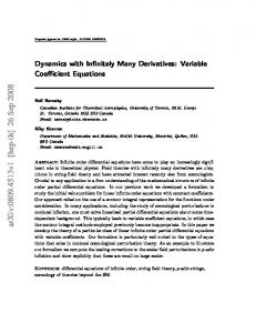
is the Schur complement of the matrix AII in A, and is usually referred to as the Schur complement matrix. The reduced system (2.3) is usually solved via a preconditioned conjugate gradient (PCG) method as the Schur complement matrix inherits the symmetric positive definitiveness property from A. To describe the Schur complement preconditioners, we need to define a partition of B. Let Vi be the singleton sets that contain one index related to one cross point (where two or more edges meet) and let V = ∪i Vi be the set with all those indices; each cross point is represented by an × in Figure 2.1. We define each edge by considering neighboring subdomains Ωj and Ωl for j 6= l, (j, l) ∈ {1, 2, . . . , N }2 where subdomain j and l are neighboring if ∂Ωj ∩ ∂Ωl is nonempty and contains at least one point not in V . We define each edge Ei by Ei = (∂Ωj ∩ ∂Ωl ) \ V. In Figure 2.1, the points belonging to the m edges (Ei )i=1,m are represented by •. We can thus describe the set B as m [ B = ( Ei ) ∪ V, (2.4) i=1

2

Fig. 2.1. A 4 × 4 box-decomposition with edge (•) and vertex (×) points.

consisting of m edges and the cross points. We now consider BPS-like preconditioners [1]. In this paper, we choose the BPS* method [4]. This scheme is closely related to the classical BPS algorithm and so serves as a good representative of BPS-like methods. It is important to understand that the operator dependent interpolation discussed in this paper is not limited to this specific BPS* method and is applicable to any BPS variant. The BPS* preconditioner can be briefly described as follows. We first define a series of projection and interpolation operators. Specifically, for each Ei we define an |Ei | × |B| matrix1 , Ri = REi , as the standard point-wise restriction (or injection) of nodal values to Ei . Its transpose extends grid functions in Ei by zero on the rest of the interface B. Similarly we define the |V |×|B| matrix, RV , as the canonical restriction to V . Thus, we set Sij ≡ Ri SRjT and SV ≡ RV SRVT . To complete the two-level preconditioner, a coarse grid operator must be defined. Assume that Ω1 , ..., ΩN form the elements of a coarse grid mesh, τ H , with mesh size H. That is, a coarse grid mesh point, Vˆj , is associated with each fine grid vertex point, Vj , and two coarse grid points, Vˆj and Vˆk , are adjacent if and only if there is an Ei that connects their corresponding fine grid points, Vj and Vk . An interpolation operator is defined by injecting coarse grid values to the corresponding fine grid cross points and performing linear interpolation for each adjacent pair of coarse grid points along the edge connecting them. This linear interpolation operator is denoted RlT . Rl is a projection operator and is the transpose of the interpolation operator. Finally, AH,l is the Galerkin coarse grid operator AH,l = Rl ARlT defined on τ H . With these notations the BPS* preconditioner is defined by X MBP S∗ = RiT Sii−1 Ri + RlT A−1 H,l Rl ,

(2.5)

(2.6)

Ei

as described in [4]. Within this paper we consider the use of Sii−1 to simplify the comparisons between methods. However, it should be noted that within practical computations, Sii−1 is typically replaced with an inexpensive spectrally equivalent approximation (e.g. [16]). This preconditioner (2.6) can be interpreted as a generalized block Jacobi scheme for the Schur complement system (2.3) where the block diagonal preconditioning for SV V is omitted and a coarse grid correction is added. The coarse grid term RlT A−1 H,l Rl incorporates global coupling between distant interfaces. 1 |.|

denotes cardinality. 3

This global coupling is critical for scalability. In particular, it has been shown in [1] that when applying the original BPS technique to a uniformly elliptic operator, the preconditioned system has a condition number κ(MBP S S) = O(1 + log2 (H/h))

(2.7)

where h is the mesh size. This result can be extended to the situation of discontinuous coefficients under the assumption that the jumps occur at interfaces between subdomains [1]. In this paper, we replace AH,l by A˜H,l = Rl SRlT .

(2.8)

It has been shown [1, 16] that in general for elliptic problems the operator AH,l is spectrally equivalent to A˜H,l (in fact they are equal in some situations) and so it is possible to use either AH,l or A˜H,l . In this text, we address only problems for which this spectral equivalence between (2.5) and (2.8) is ensured. We generally find A˜H,l more robust when highly discontinuous coefficients are present and so we use (2.8) for our convergence experiments though within practical computations AH,l may be more attractive. Thus, a linear interpolation modified BPS* scheme is given by X ˜ BP S∗,l = M RiT Sii−1 Ri + RlT A˜−1 (2.9) H,l Rl . Ei

This method will be compared to a preconditioner using operator dependent interpolation. Specifically, a specialized interpolation transfer (operator dependent) that addresses jumps that are not aligned with subdomain boundaries is defined in the next section. This operator is denoted Rod and replaces Rl yielding an operator dependent version of a BPS* scheme X T ˜−1 ˜ BP S∗,od = M RiT Sii−1 Ri + Rod AH,od Rod (2.10) Ei

where T A˜H,od = Rod SRod .

2.1. Operators Dependent Interpolation. When uniform rectangular subdomains are used on a two-dimensional structured mesh, all the edges Ei are aligned T either with the x or the y axis. In this case, interpolation, Rod , reduces to a series of one-dimensional interpolations along either x or y grid lines. Therefore, we begin by considering one-dimensional interpolation. Clearly grid points on each straightline that contain edges can be mapped to points on a line on the interval (0,1). We, therefore, consider the one dimensional model problem  d d   − (a(x) u(x)) = f in (0,1),  dx dx (2.11)    u(x) = 0 at x=0 and 1.

In the discussion that follows, we will assume that A is discretized via linear finite elements in order to simplify the presentation. Let H 1 (0, 1) be the standard Sobolev 4

space on the interval (0,1) and H01 (0, 1) its subspace whose functions vanish at x = 0 and x = 1. Given a grid xhj = jh, j = 0, ..., n on (0,1), define the fine grid linear finite element space to be V h = {v h ∈ H01 (0, 1) : v h is linear on [xhj , xhj+1 ], j = 0, ..., n − 1}, n−1 and denote the set of nodal basis functions by {φhj }j=1 ∈ V h where

φhj (xhk )

=



1 if k = j, 0 if k 6= j.

Note that the φhj ’s span V h . Let (xH i )i=1,m be the set of coarse grid points defined by the interfaces generated when partitioning (0, 1) into m + 1 non-overlapping subh domains. Define the coarse subspace V H = span{φH i ∈ V : i = 1, . . . , m} where the coarse grid nodal basis functions satisfy  1 if k = j, H H φj (xk ) = 0 if k 6= j. h h Note that the φH i ’s are linear on [xj , xj+1 ] and are not yet fully specified. Since the h h {φi } are linearly independent and the {φH i } lie in V , there exists a unique matrix R of size m × (n − 1) such that H h h T [φH 1 ...φm ] = [φ1 ...φn−1 ]R .

Thus, defining the φH i ’s is equivalent to building a restriction operator, R, and a corresponding interpolation operator, RT . We depict in Figure 2.2 an example of a coarse grid basis function that defines linear interpolation. If we denote u ˜ ∈ Vh as the linear interpolant of the function

1

....., .. . ....

,

,

,

s

h xH 1 x4

,

,

s

xh5

,bb ,

......... . ..

b

b

s

h xH 2 x6

φH 2 b

b

s

xh7

b

b b s b............

xh8

xH 3

Fig. 2.2. coarse grid basis function φH 2 associated with the linear interpolation.

˜ is discontinuous at points where a() is discontinuous. u ∈ VH , the product a ∂ u ∂x ˜ is undesirable as this term is further differentiated Intuitively, the discontinuity of a ∂ u ∂x ˜ can also be motivated using energy in (2.11). The undesirablity of a discontinuous a ∂ u ∂x minimization arguments (normally used in algebraic multigrid discussions [13]). In particular, the coarse grid system should correct smooth error components, e. These smooth components are typically characterized by small energy. That is,  where A is scaled so ||A|| = 1 and defines the usual vector inner product. ˜ implies that a high energy error correction will be However, the discontinuity of a ∂ u ∂x applied. That is, is large where u ˜ is the interpolated coarse grid correction. This is clearly contrary to what is needed and so the interpolation must be remedied 5

to yield a low energy correction. To build an interpolation operator that ensures the ˜ even if a() is discontinuous, we define a new set of coarse grid basis continuity of a ∂ u ∂x functions (and thus a new grid transfer operator). These are defined by solving the H local problems in [xH i−1 , xi ] : −

d d H (a(x) φH ) = 0 in [xH i−1 , xi ] dx dx i

(2.12)

with H φH i (xi−1 ) = 0

H φH i (xi ) = 1.

and

In Figure 2.3, we depict the basis function φH 2 when the function a() is piecewise constant with discontinuities at xh5 and xh7 .

1

" " " ....." ... s .......

xH 1

xh4

" "

H l  l φ2  l l 

s

xh5

.......... .. ..

s

xh6 xH 2

a(x) l la a s

xh7

aa s a a..............

xh8

xH 3

Fig. 2.3. coarse grid basis function φH 2 associated with the operator-dependent interpolation.

The operator-dependent interpolation is numerically constructed by solving the linear system arising from the discretization of (2.12) on each Ei . That is, interpolation for the two dimensional problem is built by solving a series of one dimensional problems (one for each subdomain interface). Each one dimensional horizontal edge problem is constructed by taking a(x, y) in (2.1) and restricting it (injection) to the proper edge thereby defining a(x) in (2.12). A similar procedure is performed on vertical edges using b(x, y). While we use injection, a(x) could also be defined by averaging a(x, y) within a neighborhood of the interface. This averaging would attempt to more accurately capture composite behavior. We have explored several different averaging procedures and have not found these worthwhile. Averaging usually does not significantly improve convergence (except on carefully contrived examples) and costs more to compute. For these reasons we do not explore averaging further in this paper. The discretization of each one dimensional PDE (2.12) yields a tridiagonal linear system with the following structure when the Dirichlet boundary conditions are included among the unknowns:   1 0  ..  .. ..  .  . .    1 + a 1) 1 1 (a −a −a Ai =  (2.13) `− 2 `+ 2 `+ 2 `− 2     . . . .. .. ..   0 1 where the (` + 1)-th row is associated with the `-th interior vertex on Ei and Z xh` a(x) 5 φh`−1 5 φh` . a`− 21 = xh `−1

6

Lemma 1. The operator-dependent interpolation reduces to linear interpolation when a ≡ 1. Proof H H H When a() ≡ 1, the solution to (2.12) such that φH i (xi−1 ) = 0 and φi (xi−1 ) = 1 is φH i =

x − xH i−1 H xH − x i i−1

which is the straight line that defines linear interpolation as depicted in Figure 2.2.  Lemma 2. The one dimensional operator-dependent interpolation defined by the solution of (2.12) reduces to the multigrid energy minimization approach [18] or to the multigrid operator-dependent interpolation when every other point is a coarse point (i.e. each subdomain contains only one point). Lemma 3. This new interpolation defines a partition of unity. That is, T 1V = 1 B , Rod

(2.14)

where the symbol 1V denotes the vectors of all 1’s on the coarse grid and 1B is the vector of 1’s on all the subdomain edges and cross points. Proof P P H H It is enough to show that i φH i (x) = 1. That is, let ψ (x) = i φi (x). Using (2.12) with 1 ≤ i ≤ m, it follows that  d d H   − (a(x) ψiH ) = 0 in [xH i−1 , xi ] dx dx   H H ψi (xi−1 ) = 1, ψiH (xH i ) = 1.

H Clearly, ψ H = 1 is a solution and by uniqueness, ψ H ≡ 1 on [xH i−1 , xi ] and the result follows.  It should be noted that this proof is essentially identical to the one given in [18, p. 1637] for Lemma 3.2 with the exception that here the number of fine grid points within H [xH i−1 , xi ] is arbitrary. This partition of unity is generally critical for good numerical convergence and occurs in most multilevel methods: the Neumann-Neumann and balancing Neumann-Neumann preconditioner [9, 10], etc. Connections between this grid transfer and standard operator dependent multigrid transfers can be found in [7].

2.2. Numerical experiments. To evaluate the sensitivity of the preconditioners to discontinuity, we consider (2.1) where the coefficients a() and b() are defined in several different ways. In all of our examples, these diffusion coefficients are piecewise constant functions. For the first two problems a() and b() are given by  in R3 ,  1 2 10 in R2 ∪ R4 , - Problem SD-F1: a() = b() =  −2 in R1 ∪ R5 .  10 in R3 ,  1 3 - Problem SD-F2: a() = b() = 10 in R2 ∪ R4 ,  −3 10 in R1 ∪ R5 . where the R’s are given by Figure 2.4. The third problem uses 7

  10−1 a() = b() = 10−2  101

- Problem SD-R:

in in in

R1 , R2 , R3 ∪ R 4 ∪ R 5 ∪ R 6 .

where the R’s are given by Figure 2.5. For sake of completeness we also consider the classical Poisson problem defined by a() = b() = 1. @

@ @

R1

@ @ @ R2 @@ R3

@

R3 @ @

R5 @

R4

R4

R1

R5

R6

R2

@

@ @ @ Figure 2.4: Example 1 - Flag

Figure 2.5: Example 2 - Region

For all these experimental results, structured meshes are used along with uniform square subdomains. The convergence of the preconditioned conjugate gradient method is attained when the 2-norm of the residual normalized by the 2-norm of the right hand side is less than 10−8 . The experiments were run on the ASCI Red machine. In all these simulations, each subdomain is assigned to a different processor and the coarse grid problem is replicated on each processor. More details on the parallel implementation can be found in [17]. We study the numerical scalability of the preconditioners by investigating the dependence of the convergence on the number of the subdomains while keeping constant the number of grid points per subdomain (i.e. 256 × 256 mesh for each subdomain, that is H h = 256). The initial guess x0 for the conjugate gradient iterations is the null vector and the righthand side is given by a constant vector. In Table 2.1, we give the results for the Poisson problem. As expected, the behavior of the two variants does not depend on the number of subdomains as predicted by (2.7) and as indicated by Lemma 1. In Table 2.2 we report the number of iterations on heterogeneous problems. Notice that for the test examples the discontinuities in the coefficients a() and b() are not aligned with the interface of the square subdomains and consequently no theory ˜ BP S∗,l is less efficient than M ˜ BP S∗,od . Further, applies. These results reveal that M ˜ BP S∗,od is numerically scalable (as is M ˜ BP S∗,l ) and follows a behavior predicted M by (2.7) even though this theory does not apply. 3. Generalization to unstructured meshes. 3.1. Definition of the interpolation operator. For unstructured meshes, the interfaces between subdomains are not necessarily aligned with either the x or y axis. Therefore, the one-dimensional PDE solution procedure involving either the coefficient function a() or b() to define (2.12) cannot be used anymore. However, we can still construct a linear system similar to (2.13) to build an interpolation operator. In particular for each interface, we consider all the elements containing an edge along the interface. For each element, we take its stiffness matrix and algebraically eliminate (i.e. reduce out) all unknowns that do not lie on the interface. Then, for each interface a matrix is assembled that includes contributions from all its reduced stiffness matrices. Finally, the two matrix rows corresponding to the end points (i.e. the two coarse grid points) are replaced by Dirichlet boundary conditions. It is important to notice that 8

# subdomains ˜ BP S∗,l M ˜ BP S∗,od M

4× 4 13 13

8× 8 17 17

16 × 16 17 17

32 × 32 15 15

Table 2.1 # iterations to solve the Poisson problem on structured meshes.

# subdomains ˜ BP S∗,l M ˜ MBP S∗,od # subdomains ˜ BP S∗,l M ˜ BP S∗,od M # subdomains ˜ BP S∗,l M ˜ MBP S∗,od

SD-F1 problem 4× 4 8 × 8 16 × 16 26 33 32 22 22 27 SD-F2 problem 4× 4 8 × 8 16 × 16 28 36 36 23 24 31 SD-R problem 4× 4 8 × 8 16 × 16 18 35 37 17 24 22

32 × 32 32 23 32 × 32 38 26 32 × 32 37 19

Table 2.2 # iterations to solve PDEs with discontinuities on structured meshes.

by reducing out the noninterface unknowns, a tridiagonal matrix is obtained. We depict in Figure 3.1 an example interface for an unstructured mesh. The shaded elements are those used to construct the tridiagonal system. For the interpolant corresponding to the left coarse grid point, the right hand side contains a ‘one’ at the left Dirichlet condition, a ‘zero’ at the right Dirichlet condition and ‘zeros’ for all other equations. Notice that this linear system effectively coincides to the original PDE on a strange domain with Neumman boundary conditions everywhere except at the two end points where Dirichlet boundary conditions are enforced. This use of local stiffness matrices has been found beneficial in other multilevel methods such as the AMGe algebraic multigrid algorithm [2], the FETI method [6], and the balancing NeummanNeumman scheme [10]. In all of these algorithms, the local stiffness matrices provides a local submatrix which is closely connected to the original physical problem (e.g. a substructure).

Fig. 3.1. An interface on unstructured meshes.

Lemma 4. The operator-dependent interpolation constructed on unstructured meshes defines a partition of the unity. 9

Proof Let A(s) be the elementary k × k stiffness matrix associated with element s. This matrix has the form   A`` A`e A(s) = Ae` Aee where the first block of rows are associated with noninterface nodes and the second block of rows correspond to the interface. For any element, s, the rank of A (s) is equal to k − 1 and its null space is spanned by the constant vector (i.e. A(s) 1k = 0k ). This implies that the local Schur complement Aee − Ae` A−1 `` A`e is also rank deficient with a null space still spanned by the constant vector. Clearly, this continues to hold when assembling the reduced stiffness matrices. That is, any constant vector is a solution to the assembled reduced system with a zero righthand side and no Dirichlet boundary conditions. Imposing Dirichlet boundary conditions equal to one at the endpoints (i.e. interpolating the coarse grid vector 1V ) forces the unique solution to be the vector of all ones along the interface.  Remark 1. On structured meshes decomposed into uniform rectangles, the above definition leads to the same operator-dependent interpolation defined in the previous section for structured meshes. While our algorithm eliminates noninterface nodes at the elementary level (i.e. before assembling), this elimination could be done after assembling. This would correspond to defining interpolation as the solution of  ∂ (a(x, y) ∂v ) − ∂ (b(x, y) ∂v ) = 0 on ˆ  − ∂x Ω,  ∂x ∂y ∂y     ∂v = 0 on  ˆ \{Vi , Vj },  ∂Ω ∂~n (3.1)  v = 1 at {Vi }       v = 0 at {Vj } 

ˆ is the union of the elements that have an edge along the interface and {Vi , Vj } where Ω refers to the two cross points corresponding to the edge endpoints (see Figure 3.1). This possibility has not been explored. Our experiences with averaging on structured meshes lead us to believe that possible benefits do not outweigh the additional costs.

3.2. Numerical experiments. To investigate the robustness and the scalability of the preconditioners we consider three model problems by defining the diffusion coefficients a() and b() in (2.1) as piecewise constant functions in (−1, 1)2 as depicted in Figures 3.2, 3.3 and 3.4. Using these notations we define a set of model problems with discontinuous coefficients as follows:  10−2    102 - Problem UD-B: a() = b() = 10−3    103

in in in in 10

R1 ∪ R 7 , R2 ∪ R 6 , R3 ∪ R 5 , R4 ;

eplacements

eplacements

R1 R2 R3 R

5

R6 R7

Fig. 3.2. Example 3 - Band.

PSfrag replacements

R4

R1 R2 R3 R4 R5 Fig. 3.3. Example 4 - Radar.

R1

R6

Fig. 3.4. Example 5 - Ring.

where the Ri are defined in Figure 3.2,  10−3      102 - Problem UD-Ra: a() = b() = 10   10−2    10−1

where the Ri are defined in Figure 3.3,  3   102   10      101 - Problem UD-Ri: a() = b() = 10−3   10−1     1    10−1

in in in in

R1 , R2 , R3 , R4 , elsewhere;

in in in in in in

R1 , R2 , R3 , R4 , R5 , R6 , elsewhere;

where the Ri are defined in Figure 3.4. The rings are labeled consecutively starting with the innermost ring labeled as R1 . We consider the following geometries and unstructured meshes to study the scalability of the preconditioners: rsq

Each subdomain is a rounded square as depicted in Figure 3.5 (i.e. a square where the sides have been replaced by arcs except on the domain boundary). 11

par

Each subdomain is a parallelogram (see Figure 3.6).

rpar

Each subdomain is a “rounded parallelogram” as depicted in Figure 3.7 (i.e. a parallelogram where the sides have been replaced by arcs except on the domain boundary).

Note that all the meshes preserve the external domain geometry. That is, the entire 1

1

0.8

0.8

0.6

0.6

0.4

0.4

0.2

0.2

0

0

−0.2

−0.2

−0.4

−0.4

−0.6

−0.6

−0.8

−1 −1

−0.8

−0.8

−0.6

−0.4

−0.2

0

0.2

0.4

0.6

0.8

−1 −1

1

Fig. 3.5. rsq unstructured mesh: a 4 × 4 decomposition.

−0.8

−0.6

−0.4

−0.2

0

0.2

0.4

0.6

0.8

1

Fig. 3.6. par unstructured mesh: a 4×4 decomposition.

1

0.8

0.6

0.4

0.2

0

−0.2

−0.4

−0.6

−0.8

−1 −1

−0.8

−0.6

−0.4

−0.2

0

0.2

0.4

0.6

0.8

1

Fig. 3.7. rpar unstructured mesh: a 4 × 4 decomposition.

composite domain Ω remains the same when the number of subdomains changes. The mesh generation and the finite element discretization of (2.1) are done us˜ BP S∗,od costs a little ing MATLAB’s PDE toolbox. In our implementation, building M ˜ bit more than constructing MBP S∗,l due to a couple of additional nearest neighbor communications. The computational cost for applying both methods, however, is identical. Solutions are obtained in parallel on the ASCI Red machine. Even though on unstructured meshes it is more difficult to control the ratio H h , we attempt to keep it constant as well as maintain a good aspect ratio for the subdomains. Therefore, we can still study the scalability of the preconditioners varying the number of subdomains while the ratio H h remains the same. Table 3.1 gives the range of number of points per subdomain for each mesh. We first report in Table 3.2 the numerical behavior of the two preconditioners for the Poisson problem. It can be observed that for that problem, the two preconditioners have similar convergence behavior. In addition the convergence is independent of the 12

Domain Decomposition Parallelograms (par) Round Squares (rsq) Round Parallelograms (rpar)

approx. range of pts/sd 890 - 900 710 - 860 780 - 1100

Table 3.1 Approximate range of points per subdomain for the considered domain decompositions.

Round square mesh (rsq) # subdomains 4× 4 8 × 8 16 × 16 ˜ BP S∗,l 16 17 16 M ˜ BP S∗,od M 18 18 17 Parallelogram mesh (par) # subdomains 4× 4 8 × 8 16 × 16 ˜ BP S∗,l M 14 14 13 ˜ BP S∗,od 14 14 13 M Round parallelogram mesh (rpar) # subdomains 4× 4 8 × 8 16 × 16 ˜ 20 19 18 MBP S∗,l ˜ BP S∗,od 21 21 20 M Table 3.2 # iterations to solve the Poisson problem on unstructured meshes.

number of subdomains as predicted by (2.7). In Tables 3.3-3.5 we report the number ˜ BP S∗,l and M ˜ BP S∗,od on discontinuous problems discretized of PCG iterations for M on unstructured meshes. For each mesh, we vary the number of subdomains from 16 ˜ BP S∗,od performs much better than M ˜ BP S∗,l ; around to 256. As it can be observed, M 50% less iterations on average for 256 subdomains. It should be mentioned that both methods have the same computational complexity per iteration and that the extra set-up time to build the operator-dependent interpolation (tridiagonal solutions) is negligible. 4. Concluding remarks. We proposed a new interpolation operator to define a closely related variant of the BPS* preconditioner. This operator-dependent interpolation is designed to tackle problems where the PDEs coefficients are either discontinuous or have large variation along the interfaces between the subdomains. The definition of this interpolation is natural on structured meshes with uniform rectangular subdomains and we proposed a generalization to unstructured meshes. This generalization preserves the constant function while taking into account possible discontinuities. The unstructured grid interpolation was inspired by AMGe and also by the fact that it reduces to the original operator dependent interpolation on uniform meshes. In this paper, we have considered the two dimensional case in order that it be fully understood first. These techniques could be used to modify BPS-like preconditioners for three dimensional problems. The key issue in three dimensions is that the subdomain interfaces are faces and so the one dimensional interpolation must be generalized to two dimensions. This would correspond to taking the elementary stiffness matrices adjacent to the faces and reducing out noninterface unknowns. The operator dependent interpolation is then determined by solving the resulting two dimensional 13

D-B problem 4× 4 8× 8 27 41 18 17 D-Ra problem # subdomains 4× 4 8× 8 ˜ BP S∗,l 31 38 M ˜ MBP S∗,od 20 23 D-Ri problem # subdomains 4× 4 8× 8 ˜ BP S∗,l M 32 44 ˜ BP S∗,od 13 15 M # subdomains ˜ BP S∗,l M ˜ MBP S∗,od

16 × 16 35 16 16 × 16 42 23 16 × 16 33 16

Table 3.3 # iterations to solve PDEs with discontinuities on unstructured round square mesh (rsq).

D-B problem # subdomains 4× 4 8× 8 ˜ BP S∗,l 22 30 M ˜ BP S∗,od M 18 20 D-Ra problem # subdomains 4× 4 8× 8 ˜ BP S∗,l M 24 40 ˜ 21 19 MBP S∗,od D-Ri problem # subdomains 4× 4 8× 8 ˜ BP S∗,l M 21 27 ˜ BP S∗,od 15 17 M

16 × 16 31 12 16 × 16 38 21 16 × 16 32 15

Table 3.4 # iterations to solve PDEs with discontinuities on unstructured parallelogram mesh (par).

D-B problem 4× 4 8× 8 30 34 22 21 D-Ra problem # subdomains 4× 4 8× 8 ˜ 31 50 MBP S∗,l ˜ BP S∗,od 25 25 M D-Ri problem # subdomains 4× 4 8× 8 ˜ BP S∗,l M 28 38 ˜ 22 26 MBP S∗,od # subdomains ˜ BP S∗,l M ˜ BP S∗,od M

16 × 16 37 20 16 × 16 52 35 16 × 16 45 22

Table 3.5 # iterations to solve PDEs with discontinuities on unstructured round parallelogram mesh (rpar).

14

PDE discretizations on each face. Given the connections to AMGe which has been developed for three dimensional problems, we anticipate that this would yield an effective method. Unlike AMGe, however, complications associated with applying the algorithm on coarser grids recursively do not arise due to the two-level nature of these domain decomposition preconditioners. Extensive experiments illustrate the numerical scalability of the BPS* method on discontinuous coefficient problems even though assumptions used to develop the theory are violated. In practice both linear interpolation as well as operator dependent interpolation yield scalable methods. While both are scalable, however, the operator dependent scheme significantly outperforms the linear interpolation method with similar computational complexity. REFERENCES [1] J. Bramble, J. Pasciak, and A. Schatz, The construction of preconditioners for elliptic problems by substructuring I., Math. Comp., 47 (1986), pp. 103–134. [2] M. Brezina, A. Cleary, R. Falgout, V. Henson, J. Jones, T. Manteuffel, S. McCormick, and J. Ruge, Algebraic multigrid based on element interpolation (AMGe), SIAM J. Sci. Comput., 22 (2000), pp. 1570–1592. [3] L. Carvalho, L. Giraud, and P. L. Tallec, Algebraic two-level preconditioners for the Schur complement method, SIAM J. Sci. Comput., 22 (2001). [4] T. Chan and T. Mathew, Domain Decomposition Algorithms, vol. 3 of Acta Numerica, Cambridge University Press, Cambridge, 1994, pp. 61–143. [5] M. Dryja, B. Smith, and O. Widlund, Schwarz analysis of iterative substructuring algorithms for elliptic problems in three dimensions, SIAM J. Numer. Anal., 31 (1993), pp. 1662–1694. [6] C. Farhat and F.-X. Roux, A method of finite element tearing and interconnecting and its parallel solution algorithm, Int. J. Numer. Meth. Engng., 32 (1991), pp. 1205–1227. [7] L. Giraud and R. S. Tuminaro, Grid transfer operators for highly variable coefficient problems, Tech. Rep. TR/PA/93/37, CERFACS, Toulouse, France, 1993. Available on www.cerfacs.fr/algor/algo reports. [8] A. Klawonn and O. B. Widlund, FETI and Neumann-Neumann iterative substructuring methods: connections and new results, Comm. Pure Appl. Math., LIV (2001), pp. 57–90. [9] P. Le Tallec, Domain decomposition methods in computational mechanics, vol. 1 of Computational Mechanics Advances, North-Holland, 1994, pp. 121–220. [10] J. Mandel, Balancing domain decomposition, Communications in Numerical Methods in Engineering, 9 (1993), pp. 233–241. [11] J. Mandel and M. Brezina, Balancing domain decomposition for problems with large jumps in coefficients, Mathematics of Computation, 65 (1996), pp. 1387–1401. [12] J. Mandel and R. Tezaur, Convergence of substructuring method with Lagrange multipliers, Numer. Math., 73 (1996), pp. 473–487. ¨ben, Algebraic multigrid, in Multigrid Methods, S. McCormick, ed., Fron[13] J. Ruge and K. Stu tiers in Applied Mathematics, Philadelphia, 1987, SIAM, pp. 73–130. [14] B. Smith, Domain Decomposition Algorithms for the Partial Differential Equations of Linear Elasticity, PhD thesis, Courant Institute of Mathematical Sciences, Sept. 1990. Tech. Rep. 517, Department of Computer Science, Courant Institute. [15] , A domain decomposition algorithm for elliptic problems in three dimensions, Numer. Math., 60 (1991), pp. 219–234. [16] B. Smith, P. Bjørstad, and W. Gropp, Domain Decomposition, Parallel Multilevel Methods for Elliptic Partial Differential Equations, Cambridge University Press, New York, 1st ed., 1996. [17] F. G. Vasquez, Internship report on domain decomposition methods for the solution of partial differential equations, Technical Report TR/PA/00/98, CERFACS, Toulouse, France, 2000. Available on www.cerfacs.fr/algor/algo reports. [18] W. L. Wan, T. F. Chan, and B. Smith, An energy-minimizing interpolation for robust multigrid, SIAM J. Sci. Comput., 21 (2000), pp. 1632 – 1649. [19] O. Widlund, Iterative substructuring methods: Algorithms and theory for elliptic problems in the plane, in First International Symposium on Domain Decomposition Methods for Partial Differential Equations, R. Glowinski, G. Golub, G. Meurant, and J. P´eriaux, eds., Philadelphia, PA, 1988, SIAM. 15