Fast GBA. GBA. AIM. Hou. GBVS. Itti. Judd. AWS. LG. Spec. Erdem. Fig. 1. Figure shows a test image (from database [12]) and the associated the saliency maps ...
Group Based Asymmetry–A Fast Saliency Algorithm Puneet Sharma, and Oddmar Eiksund Department of Engineering and Saftey(IIS), UiT-The Arctic University of Norway, Tromsø, Norway.
Abstract. In this paper, we propose a saliency model that makes two major changes in a latest state-of-the-art model known as group based asymmetry. First, based on the properties of the dihedral group D4 we simplify the asymmetry calculations associated with the measurement of saliency. This results is an algorithm which reduces the number of calculations by at-least half that makes it the fastest among the six best algorithms used in this paper. Second, in order to maximize the information across different chromatic and multi-resolution features the color image space is de-correlated. We evaluate our algorithm against 10 state-of-the-art saliency models. Our results show that by using optimal parameters for a given data-set our proposed model can outperform the best saliency algorithm in the literature. However, as the differences among the (few) best saliency models are small we would like to suggest that our proposed model is among the best and the fastest among the best.
1
Introduction
In literature, visual attention has been mainly classified as: top-down, and bottomup [16]. Top-down, is voluntary, goal-driven, and slow, i.e., usually in the range between 100 milliseconds to several seconds [16]. It is assumed that the top-down attention is closely linked with cognitive aspects such as memory, thought, and reasoning. For instance, by using top-down mechanisms we can read this text one word at a time, while neglecting other aspects of the scene such as, words in other lines. In contrast, bottom-up attention (also known as visual saliency) is associated with attributes of a scene that draw our attention to a particular location. These attributes include: motion, contrast, orientation, brightness, and color [13]. Bottom-up mechanisms are involuntary, and faster as compared to top-down [16]. For instance, a red object among green objects, and an object placed horizontally among vertical objects are some stimuli that would automatically capture our attention in the environment. In a recent study by Alsam et al. [1,2] it was proposed that asymmetry can be used as a measure of saliency. In order to calculate asymmetry of an image region the authors used dihedral group D4 , which is the symmetry group of the square. D4 consists of 8 group elements namely, rotation by 0, 90, 180 and 270
2
Puneet Sharma, and Oddmar Eiksund
degrees and reflection about the horizontal, vertical and two diagonal axes. The saliency maps obtained from their algorithm show good correspondence with the saliency maps calculated from the classic visual saliency model by Itti et al. [11]. Inspired by the fact that bottom-up calculations are fast, in this paper, we use the symmetries present in the dihedral group D4 to make the calculations associated with the D4 group elements simpler and faster to implement. In doing so, we modify the saliency model proposed by Alsam et al. [1,2]. For details, please see section 2. Next, we are motivated from the study by Garcia-Diaz et al. [8] which implies that in order to quantify distinct information in a scene, our visual system decorrelates its chromatic and multi-resolution features. Based on this, we perform the de-correlation of input color image by calculating its principal components (details in section 2.3).
2 2.1
Method Background
Alsam et al. [1,2] proposed a saliency model that uses asymmetry as a measure of saliency. In order to calculate saliency, the input image is decomposed into square blocks, and for each block the absolute difference between the block itself and the result of the D4 group elements acting on the block is calculated. The sum of the absolute differences (also known as L1 norm) for each block is used as a measure of asymmetry for the block. The asymmetry values for all the blocks are then collected in an image matrix and scaled up to the size of original image using bilinear-interpolation. In order to capture both the local and the global salient details in an image three different image resolutions are used. All maps are combined linearly to get a single saliency map. In their algorithm, asymmetry of a square region is calculated as follows: M (i.e., the square block) is defined as an n × n-matrix and σi as one of the eight group elements of D4 . The eight elements are the rotations along 0◦ , 90◦ , 180◦ and 270◦ , and the reflections along horizontal, vertical and two diagonal axis of the square. Asymmetry of M by σi is denoted by A(M ) to be, A(M ) =
8 X
||M − σi M ||1 ,
(1)
i=1
where ||1 represents L1 norm. Instead of calculating asymmetry value associated with each group element and followed by their sum, we believe that the algorithm can run faster if the calculations in equation 1 are made simpler. For this we propose a fast implementation of these operations pertaining to the D4 group elements. 2.2
Fast implementation of the group operations
Let us assume M as 4 by 4 matrix,
Lecture Notes in Computer Science
M =
α1 a
b β1
c α2 β2 d e
γ2 δ2 f
γ1
g
h δ1
3
The asymmetry A(M ) of the matrix M is measured as the sum of absolute differences of the different permutations of the matrix entries pertaining to the D4 group elements and the original. The total number of such differences are determined to be 40. As the calculations associated with absolute differences are repeated for the rotation and reflection elements of the dihedral group D4 , our objective is to find the factors associated with these repeated differences. For our calculations we divide the set of matrix entries into two computational categories: the diagonal entries (highlighted in yellow) and the rest of the entries of M . Please note that these calculations can be generalized to any matrix of size n by n, given that n is even. For the rest of the entries, first, we can look at |a − b|. This element will only be possible if we flip the matrix about the vertical axis. This will result in two parts in the sum, |a − b| and |b − a|, giving a factor 2. Here a and b represents a reflection symmetric pair, and all other reflection symmetric pairs will behave in the same way. Now let’s focus on |a − d|. This represents a rotational symmetric pair. Rotating the matrix counterclockwise will move d onto the position of a giving a part |a − d| in the sum. Rotating clockwise gives us, |d − a|. As these differences are not plausible in any other way, this gives us a factor of 2. All other rotational symmetric pairs will behave in the same way. This means that the asymmetry for the rest of the entries can be calculated as follows: 2|a − b| + 2|a − c| + 2|a − d| + · · · + 2|g − h|.
(2)
For the diagonal entries, we can see that they exhibit both rotation and reflection symmetries. For instance, we can move β to the place of α and α to β with one reflection and two rotations. This gives us a factor of 4. The asymmetry of one set of diagonal entries can be calculated as follows: 4|α − β| + 4|α − γ| + 4|α − δ| + 4|β − γ| + 4|β − δ| + 4|γ − δ|.
(3)
The asymmetry for both the diagonal entries and the rest is represented as, A(M ) =
4|α1 − β1 | + 4|α1 − γ1 | + · · · + 4|γ1 − δ1 | +4|α2 − β2 | + 4|α2 − γ2 | + · · · + 4|γ2 − δ2 | +2|a − b| + 2|a − c| + · · · + 2|g − h|.
(4)
As shown in equation 4, the asymmetry calculations associated with the matrix M are reduced to a quarter for the diagonal entries and one-half for the rest of the entries. This makes the proposed algorithm at least twice as fast.
4
2.3
Puneet Sharma, and Oddmar Eiksund
De-correlation of color image channels
De-correlation of color image channels is done as follows: First, using bilinear interpolation we create three resolutions (original, half and one-quarter) of the RGB color image. In order to collect all the information in a matrix the (half and one-quarter) resolutions are rescaled to the size of original. This gives us a matrix I of size w by h by n, where w is the width of the original, h is the height and n is the number of channels (3 × 3 = 9). Second, by rearranging the matrix entries of I we create a two dimensional matrix A of size w × h by n. We do normalization of A around the the mean as, B = A − µ,
(5)
where µ is the mean for each of the channels, and B is w × h by n. Third, we calculate correlation matrix of B as, C = B T B,
(6)
where the size of C is n by n. Four, the Eigen decomposition of a symmetric matrix is represented as, C = V DV T ,
(7)
where V is a square matrix whose columns are Eigen-vectors of C and D is the diagonal matrix whose diagonal entries are the corresponding Eigen-values. Finally, the image channels are transformed into Eigenvector space (also known as principal components) as: E = V T (A − µ),
(8)
where E is the transformed space matrix which is rearranged to get back the de-correlated channels. 2.4
Implementation of the algorithm
First, the input color image is rescaled to half the original resolution. Second, by using the de-correlation procedure described in section 2.3 on resulting image we get 9 de-correlated multi-resolution and chromatic channels. Third, a fixed block size (e.g.,12) is selected– as discussed later in section 3.6, this choice is governed by the data-set. If the rows and columns of the de-correlated channels are not divisible by the block size then they are padded with neighboring information along the right and bottom corners. Finally, the saliency map is generated by using the procedure outlined in section 2.2. The code is open source and will be available at Matlab Central for the research community.
3
Comparing different saliency models
The performance of visual saliency algorithms is usually judged by how well the two-dimensional saliency maps can predict the human eye fixations for a given image. Center-bias is a key factor that can influence the evaluation of saliency algorithms [15].
Lecture Notes in Computer Science
3.1
5
Center-bias
While viewing images, observers tend to look at the center regions more as compared to peripheral regions. As a result of that a majority of fixations fall at the image center. This effect is known as center-bias and is well documented in vision studies [18,17]. The two main reasons for this are: first, the tendency of photographers to place the objects at the center of the image. Second, the viewing strategy employed by observers, i.e., to look at center locations more in order to acquire the most information about a scene [19]. The presence of center bias in fixations makes it difficult to analyze the correspondence between the fixated regions and the salient image regions. 3.2
Shuffled AU C metric
Shuffled AU C metric was proposed by Tatler et al. [18] and later used by Zhang et al. [20] to mitigate the effect of center-bias in fixations. The shuffled AU C metric is a variant of AU C [7] which is known as area under the receiver operating characteristic curve. For a detailed description of AU C, please see the study by Fawcett [7]. To calculate the shuffled AU C metric for a given image and one observer, the locations fixated by the observer are associated with the positive class (in a manner similar to the regular AU C metric), however, the locations for the negative class are selected randomly from the fixated locations of other unrelated images, such that they do not coincide with the locations from the positive class. Similar to the regular AU C, the shuffled AU C metric gives us a scalar value in the interval [0,1]. If the value is 1 then it indicates that the saliency model is perfect in predicting fixations. If Shuffled AU C