Grouping-based Interference Alignment with IA-Cell ... - CiteSeerX

1

Grouping-based Interference Alignment with IA-Cell Assignment in Multi-Cell MIMO MAC under Limited Feedback

arXiv:1409.3686v1 [cs.IT] 12 Sep 2014

Pan Cao, Student Member, IEEE, Alessio Zappone, Member, IEEE, Eduard A. Jorswieck, Senior Member, IEEE

Abstract—Interference alignment (IA) is a promising technique to efficiently mitigate interference and to enhance the capacity of a wireless communication network. This paper proposes a grouping-based interference alignment (GIA) with optimized IACell assignment for the multiple cells interfering multiple-input and multiple-output (MIMO) multiple access channel (MAC) network under limited feedback. This work consists of three main parts: 1) a complete study (including some new improvements) of the GIA with respect to the degrees of freedom (DoF) and optimal linear transceiver design is performed, which allows for lowcomplexity and distributed implementation; 2) based on the GIA, the concept of IA-Cell assignment is introduced. Three IA-Cell assignment algorithms are proposed for the setup with different backhaul overhead and their DoF and rate performance is investigated; 3) the performance of the proposed GIA algorithms is studied under limited feedback of IA precoders. To enable efficient feedback, a dynamic feedback bit allocation (DBA) problem is formulated and solved in closed-form. The practical implementation, the required backhaul overhead, and the complexity of the proposed algorithms are analyzed. Numerical results show that our proposed algorithms greatly outperform the traditional GIA under both unlimited and limited feedback. Index Terms—Interfering MIMO networks, interference alignment (IA), IA-Cell assignment, limited feedback, Grassmainn subspace quantization, dynamic feedback bit allocation.

I. I NTRODUCTION Small cells is considered the most promising technique to keep up with the exponential increase of data-rate demand foreseen for 5G networks [1]. However, more base stations (BSs) sharing the same spectrum result in increased multi-cell interference, which is a major limiting factor if not properly managed [2]. Cooperative Multi-Point (CoMP), already standardized in long term evolution advanced (LTE-A) [3], aims at turning inter-cell interference (ICI) into an advantage by letting BSs share their data and perform joint precoding/decoding. This requires the exchange of global channel state information (CSI) as well as (possibly) user data via high data rate backbone connections, which might be a problem when the BSs belong to different operators or have conflicting utilities. In these cases, coordination schemes among BSs, without global CSI and user data exchange might be feasible [4]. In this work, we consider an interfering multiple-input and multiple-output (MIMO) multiple access channel (MAC) network, which is well matched to the multi-cell multi-user uplink The authors are with the Chair of Communications Theory, Communications Laboratory, Dresden University of Technology, Dresden 01062, Germany (e-mail: {Pan.Cao, Alessio.Zappone, Eduard.Jorswieck}@tu-dresden.de)

scenario. Multiple cells share their spectrum so as to form a coordinated cluster. Each BS serves multiple users within its own cell and each node is equipped with multiple antennas. The uplink signal is corrupted by both ICI and inter-user interference (IUI). In order to eliminate both interference, the linear transceiver with simple implementations is preferred. This was addressed in [5] by applying a coordinated zeroforcing (ZF) scheme to mitigate both IUI and ICI in the interfering MIMO broadcast channel (BC). However, ZF alone fails if a BS does not have sufficient antennas or if degrees of freedom (DoF) maximization is the goal. With this respect, a well-established technique called interference alignment (IA) is helpful [6], [7]. IA is applied to suppress the interference at a given receiver, thereby reducing the number of antennas required to implement ZF reception [8]. IA for DoF and sumrate optimization in K-user MIMO interference channel is considered in [9]–[11] by designing the linear IA precoders and decoders. Generally, it is difficult to obtain the closed-form linear IA transceiver and iterative algorithms based on global CSI are usually required, except for the special case of square and invertible channel matrices, e.g. in [9]. More recently, IA has been applied to MIMO cellular networks. In [12], a multicell MIMO downlink channel is studied and a distributed IA algorithm is proposed to suppress or minimize the interference to non-intended users. Also, [13] develops an IA technique for a downlink cellular system with CSI-exchange and feedback within each cell. In [14], [15], conditions for the feasibility of IA and DoF for MIMO cellular networks are investigated. To reduce the complexity and CSI requirement, the concept of grouping-based IA (GIA) is proposed for a two-cell singlestream interfering MIMO-BC in [16]. The idea is to let each cell align its interference to another cell, which will then require less antennas to implement ZF reception. Moreover, the GIA enables to compute the closed-form IA transceiver based on only local CSI. This GIA is extended to a multicell interfering MIMO-BC in [17], where both the feasible condition on the GIA and a low complexity IA decoder design are studied. The implementation of IA requires a closed-loop transmission. The feedback is needed in either the downlink or the uplink scenario1 . Since the feedback links are usually 1 In the downlink, the feedback takes two phases: 1) the downlink CSI is first fed back to BSs and 2) the IA decoders designed at BSs are reported to users (also called dedicated training phase). In the uplink, the IA precoders designed at BSs based on the perfect CSIR are fed back to the users.

2

capacity-limited in realistic scenario, codebook-based feedback is widely used and already defined in modern wireless standards, e.g., in LTE [18], to reduce the feedback overhead. The idea is to map a channel matrix/vector or precoder/decoder to an index of the closest codeword in a predefined codebook known at both transmitter and receiver. The feedback of an index takes only a finite number of feedback bits, while a performance loss is inevitable because of the quantization distortion. Thus, it becomes an important issue how to control/reduce the performance loss under limited feedback [19]. For a MIMO BC with ZF precoder, the performance loss due to limited feedback is studied in [20], [21] and also with block diagonalization in [22], [23]. For a MIMO interference channel with heterogeneous path loss and spatial correlations, [24] develops a spatial codebook design and performing dynamic quantization via feedback bit allocation. In [25]–[27], the feedback bits scaling law to maintain the maximum DoF for IA on general MIMO interference networks is investigated. Motivated by this background, we focus on the GIA in a multi-cell interfering MIMO-MAC under limited feedback, answering the following fundamental questions. 1) How to design the optimal linear GIA transceiver with low complexity? We further develop previous related works (e.g. [16], [17]), providing a low-complexity restriction-relaxation approach to compute the optimal linear GIA transceivers which not only nulls out both ICI and IUI but also maximizes the rate performance. 2) How to determine a good IA-Cell assignment? By the GIA, each cell chooses to align its interference to another cell. However, this choice clearly impacts the rate performance. Optimizing the selection of the cell to/from which a given cell provides/receives the aligned interference, is a problem which was not considered in previous works. We refer to this problem as IACell assignment and provide three IA-Cell assignment algorithms: a centralized one, which yields global optimality but requires high complexity and overhead, and two distributed ones, which yield a stable or almost stable assignment with limited complexity and backhaul overhead. 3) How to efficiently feed back the GIA precoders to the transmitters? In the uplink MIMO cellular scenario, the GIA precoders need to be fed back to the users. we employ Grassmannian subspace quantization, developing a novel quantized subspace characterization which allows to derive a closed-form upper bound of the single-cell residual interference to noise ratio (RINR). Based on this bound, we formulate and solve in closedform a feedback bit allocation problem for sum-cluster RINR minimization. Furthermore, the effect of the sum feedback bit budget on the sum-cluster rate is analyzed. The three contributions above jointly provide a comprehensive holistic design of the multi-cell MIMO MAC system under limited feedback. The paper is organized as follows: a complete study of the GIA on DoF and optimal linear transceiver design is provided in Section III. In Section IV, the IA-Cell assignment problem is addressed and solved.

The limited feedback scenario is considered in Section V. In Section VI, we analyze practical implementation, backhaul overhead and complexity of the proposed GIA algorithm with optimized IA-Cell assignment and under limited feedback. The numerical results in Section VII show the effectiveness of the proposed algorithms under unlimited and limited feedback.2 II. S YSTEM M ODEL Consider a MIMO cellular environment with K cells. In each cell, a central BS simultaneously serves L users in its own cell, where each BS and each user are equipped with NB and NU antennas, respectively. In order to increase the spectral efficiency and occupancy level compared with classical FDMA and TDMA techniques, K cells form a coordinated cluster and operate over the same time-frequency resource, while the introduced IUI and ICI in return corrupt the received desired signal and limit the detection efficiency or transmission rate. Thus, interference management is required. This work focuses on the uplink scenario, where the setup is modeled as an interfering MIMO-MAC system (K, L, NB , NU , ds ). Each user i in cell k, denoted by user (i, k), transmits ds symbols xi,k ∈ Cds ×1 with E[xi,k xH i,k ] = I ds to its corresponding BS k. The symbol vector xi,k is precoded by a linear precoder V i,k ∈ CNU ×ds subject to Tr(V H i,k V i,k ) ≤ Pi,k where Pi,k is the transmit power budget. We assume that the local CSIR is perfectly estimated at each BS based on uplink pilot signals (e.g., [28]). The received signal at BS k for user (i, k) is expressed as L X H kj,k V j,k xj,k y i,k = H ki,k V i,k xi,k + {z } j=1,j6=i | desired signal {z } | IUI

+

K X

L X

ℓ=1,ℓ6=k m=1

|

H km,ℓ V m,ℓ xm,ℓ +nk , {z

ICI

(1)

}

where H ℓi,k denotes the q channel matrix from user (i, k) to ℓ H ℓ , where η ℓ BS ℓ and is modeled as ηi,k i,k i,k denotes the ℓ

effect of path-loss, and H i,k ∈ CNB ×NU is a Rayleigh fading channel matrix. Each channel is assumed to be quasi-static and frequency flat fading. nk ∈ CNB ×1 is the additive white Gaussian noise vector with zero mean and variance σk2 I NB . With the linear single-user decoding scheme, the received b i,k = signal vector y i,k for user (i, k) can be decoded as x NB ×ds . In order to make UH y by the decoder U ∈ C i,k i,k i,k efficient detection of the desired signal, the desired signal + 2 Notations: N+ denotes the nonnegative integer domain. [x] int and [x]int 0 denote the integer and the nonnegative integer around x, respectively. Give a M × 1 vector x, arglist maxm=1,...,M x generates a M × 1 vector where the elements are re-arranged in decreasing order. (·)H , rank(·) and Tr(·) denote Hermitian transpose, rank and trace, respectively. λi (X) and U X denote the i-th largest eigenvalue and the eigen-space of X, respectively. Span{X} denotes the space spanned by the column space of ∆ X. ΠX = X(X H X)−1 X H denotes the orthogonal projection onto the ∆ column space of X, and Π⊥ X = I − ΠX denotes the orthogonal projection onto the orthogonal complement of the column space of X. X ⊥ refers to the eigenvectors corresponding to the nonzero eigenvalues of I − XX H .

3

should be linearly independent of the interference, i.e., the following conditions need to be satisfied: k UH i,k H j,k V j,k = 0, k UH i,k H m,ℓ V m,ℓ k rank(U H i,k H i,k V i,k )

= 0, = ds ,

∀j 6= i

(2a)

∀ℓ 6= k, ∀m

(2b)

∀i, k,

(2c)

where (2a) and (2b) enable the mitigation of IUI and ICI, respectively, and (2c) guarantees the transmission of ds data streams per user. Then, the achievable rate for user (i, k) is Ri,k = log det(I ds +

1 H k k,H U H V i,k V H i,k H i,k U i,k ). σk2 i,k i,k (3)

For the conditions (2a)-(2c) to be fulfilled in the system (K, L, NB , NU , ds ), any user (i, k) needs to satisfy i h k k K L UH i,k {H j,k V j,k }j=1,j6=i , {F ℓ }ℓ=1,ℓ6=k ,

UH i,k F i,k

=0

(4)

NB ×(KL−1)ds

denotes the interference matrix. where F i,k ∈ C Sufficient and Necessary Conditions: (4) is fulfilled if and only if NB ≥ rank(F i,k ) + ds such that BS k could provide at least a rank(F i,k )-dimensional subspace to nullify all the interference to user (i, k) and simultaneously guarantee ds DoF per user. Due to rank(F i,k ) ≤ (KL − 1)ds , it is sufficient to fulfill (4) by only exploiting the ZF decoding if NB ≥ KLds . In general, we have rank(F i,k ) = (KL − 1)ds if no restrictions is on the transmission through Rayleigh fading channels. In this paper, we study the interference mitigation in the nontrivial case ((K − 1)L + 1)ds ≤ NB < KLds where the sole ZF decoding fails and IA is required. Instead of developing iterative IA algorithms, we deal with the problem of lowcomplexity IA transceiver design, also considering the problem of IA-Cell assignment and limited feedback. Definitions: The channel set from users in cell k to BS ℓ ℓ: H ℓk , {H ℓi,k }L , i=1 . The local CSIR of BS ℓ: H ℓ ℓ K {H k }k=1 . The interference from cell k to cell ℓ: F k , [H ℓ1,k V 1,k , . . . , H ℓL,k V L,k ] ∈ CNB ×Lds . The IUI of user k L NB ×(L−1)ds . (i, k): F IUI i,k , [{H j,k }j=1,j6=i ] ∈ C III. I NTERFERENCE A LIGNMENT AND M ITIGATION In this section, we develop a restriction-relaxation two-stage algorithm based on the GIA method proposed in [16], [17] to determine the optimal IA transceiver in closed-form. A. Feasible Conditions for the GIA The GIA method in [17] is a generalization of the noniterative grouping scheme originally proposed in [16] to completely suppress the interference. The basic idea of GIA method in [17] is to group all the users in one cell to generate a joint precoder aligning their interference to another cell. Let IA Cell k −→ Cell k ′ denote that cell k aligns its interference ′ to cell k . The feasible conditions for the GIA method and its DoF performance are shown in the following proposition.

Proposition 1 For a multi-cell interfering MIMO-MAC system (K, L, NB , NU , ds ), at least ds DoF per user and KLds sum DoF can be achieved by the GIA method if L−1 1 NB + ds and NB ≥ ((K − 1)L + 1)ds . (5) L L Proof: Without loss of generality, to fix ideas we consider the following scenario. NU ≥

IA

IA

IA

IA

Cell 1 −→ Cell 2 −→ . . . −→ Cell K −→ Cell 1.

(6)

IA

In particular, the procedure of Cell k −→ Cell k + 1 can be implemented by k+1

Fk

k+1 , Span{H k+1 1,k V 1,k } = . . . = Span{H L,k V L,k }. (7)

First, we restrict (7) to find those precoding matrices such that in k+1 in H k+1 1,k V 1,k = . . . = H L,k V L,k .

(8)

L By this restriction stage, {V in i,k }i=1 in (8) is sufficient but not necessary to (7). And, (8) is rewritten as     V in k+1 1,k H k+1 −H 0 · · · 0 in  1,k 2,k    V 2,k   .. .. .. .. ..    ..  . . . . .  .  k+1 k+1 H 1,k 0 0 ··· −H L,k in V L,k

, Ak+1 V in k =0 k Ak+1 k

(9)

in k

∈ CLNU ×ds . To where ∈ C(L−1)NB ×LNU and V in fulfill (9), the joint IA precoder V k should lie in the null space of Ak+1 , which requires LNU ≥ (L − 1)NB + ds such k that Ak+1 has a at least ds -dimensional null space. k By (9), the original Lds -dimensional interference subspace k+1 F k+1 is aligned to a ds -dimensional subspace F k because k (7) holds, while the interference F ℓk ∀ℓ 6= k, k + 1 is still with Lds dimensions. Under the assignment of (6), it is sufficient for each BS k to remove the complete interference for user (i, k) by the ZF decoding if NB ≥ ((K − 1)L + 1)ds . Remark 1 By the feasible conditions (5) in Proposition 1, we gain the following insights on system design. 1) Given (K, L, NB , NU ), each user achieves at most NB min(LNU − (L − 1)NB , (K−1)L+1 ) DoF; 2) Given (K, L, NB , ds ), each user needs at least ((L − 1)(K − 1) + 1)ds antennas to guarantee its ds DoF; 3) Given (K, NB , NU , ds ), each cell serves at most NB −ds −ds , (K−1)d ) users; min( NNBB−N U s −ds 4) Given (L, NB , NU , ds ), at most NB Lds + 1 cells can be scheduled to form a cluster with the sum DoF of KLds 1 if NU ≥ L−1 L NB + L ds . If the inequalities in both feasible conditions (5) become equalities, the required number of BS and user antennas are the smallest.  B. Transceiver Optimization for the GIA As in [17], [29], we hereafter focus on the worst-case that 1 NB = ((K − 1)L + 1)ds and NU = ⌈ L−1 L NB + L ds ⌉. In

4

this case, the optimal GIA transceiver are computed in closedform. Proposition 2 Let us define T i , [0NU ×(i−1)NU , I NU , 0NU ×(L−i)NU ]  ⊥ k+1,H V in k = Ak   n oK k IUI k F IA,k−1 , F F , F , k−1 . i,k ℓ i,k ℓ=1,ℓ6=k,k−1

(10) (11) (12)

Considering (6) and the uniform power allocation policy, the achievable rate of each user (i, k) in (3) is maximized by the optimal transceiver r Pi,k in,H H − 21 (13) T i V in T i T i V in V i,k = k (V k k ) ds  ⊥ U i,k = F IA,k−1 . (14) i,k

Proof: Without loss of generality, we consider the scek+1 nario (6). First, since V in to k lies in the null space of Ak in fulfill (9). Based on the fact Span(V i,k X) = Span(V in i,k ) where X ∈ Cds ×ds is an arbitrary full-rank matrix, the IA precoder for each user (i, k) is defined as in out out V i,k , V in i,k V i,k = T i V k V i,k

(15)

where T i is a selection matrix defined in (10) and V in k is ds ×ds is an inner precoder defined in (11), and V out i,k ∈ C an outer precoder subject to the transmit power constraint in out Tr(V out,H V in,H i,k i,k V i,k V i,k ) ≤ Pi,k , which is used to relax the restriction from (7) to (8) and this relaxation is tight. The optimal precoder V i,k can be determined by further optimizing V out i,k . in k out Also due to Span(H kj,ℓ V in j,ℓ V j,ℓ ) = Span(H j,ℓ V j,ℓ ), it is sufficient to design the ZF decoder U i,k only based on V in j,ℓ but without knowledge of V out j,ℓ . The ZF decoder for user (i, k) can be designed by  ⊥ IA,k−1 out U i,k , U in U out (16) i,k U i,k = F i,k i,k ,

where F IA,k−1 defined in (12) is a NB × ((K − 1)L + 1)ds i,k interference matrix with the aligned interference from cell k − 1. U in i,k serves as an inner decoder to nullify interferds ×ds is an outer decoding matrix with ence, and U out i,k ∈ C out,H out U i,k U i,k = I ds . With the IA transceiver in form of (15) and (16), the achievable rate of each user (i, k) becomes3   1 fk out out,H f k,H IA Ri,k = log det I ds + 2 H H i,k , (17) i,k V i,k V i,k σk k

f denotes the effective channel from (i, k) to BS k where H i,k k

f , U in,H H k T i V in , H i,k i,k k i,k

(18)

in out and with the constraints Tr(V out,H V in,H i,k i,k V i,k V i,k ) ≤ Pi,k . Under the assumption of equal transmit power allocation with

3 The

out rate RIA i,k is independent of the unitary matrix U i,k .

IA practical considerations4, maximization of Ri,k yields V out i,k = q 1 Pi,k in,H in − 2 , thereby (13)-(14). ds (V i,k V i,k ) The improvements of the derived results with respect to previous works on the GIA [16], [17] are two-fold. • Lower complexity: The complexity of the GIA mainly depends on the singular-value decomposition (SVD) of K matrices {Ak+1 }. By the new formulation (9), our GIA k takes KO((L−1)2 LNB2 NU ) arithmetic operations, since each Ak+1 is a (L − 1)NB × LNU matrix. In contrast, k [17, Eq. (27)] (same as [16]) and [17, Eq. (12)-(13), (15)] have the complexity of KO(L2 NB2 (LNU + NB ))
or K LO(NB3 + NB2 NU ) + 2(L + log2 (L))O(2NB2 NU ) , respectively. It follows that the complexity of our GIA by (9) is always lower than [17, Eq. (27)] and also lower than that by [17, Eq. (12)-(13), (15)] when L ≤ 3. 5 • Optimality/Tightness of the restriction-relaxation: The procedure of the restriction from (7) to (8) combined with the relaxation by introducing the outer precoder and in out decoder, subject to Tr(V out,H V in,H i,k i,k V i,k V i,k ) ≤ Pi,k and U out i,k being a unitary matrix, into the definitions (15) and (16) is tight. This property guarantees the optimality of linear transceiver design by the restriction-relaxation method, which does not hold in the work [17] where the constraints Tr(V out,H V out i,k ) ≤ Pi,k and the dirty-paperi,k coding scheme are adopted.

Remark 2 The GIA as a non-iterative algorithm determines the IA transceiver in a distributed way and with low complexity. For the distributed implementation, BSs need to exchange K their inner precoders {V in k }k=1 with each other, while the out outer precoder V k and the outer decoder U out can be k designed by each user (i, k) and BS k independently.  IV. IA-C ELL A SSIGNMENT P ROBLEM F ORMULATIONS AND S OLUTIONS In this section we introduce the concept of IA-Cell assignment, motivate its importance for network performance and propose three algorithms for assignment optimization. A. IA-Cell Assignment Problems IA

1) Observation and Motivation: For Cell k −→ Cell k ′ , we label cell k as the IA-provider for cell k ′ and cell k ′ as the IA-receiver from cell k. Clearly, this poses an assignment problem between IA-providers and IA-receivers – how should we select the IA-receiver (or IA-provider) corresponding to a given IA-provider (or IA-receiver)? From the perspective of spatial resources, a cell will waste part of its transmit spatial resources if it aligns its interference to other cells because of the IA constraint. On the other hand, a cell can save its 4 Instead of the optimal water-filling based power allocation across the data streams, the uniform power allocation policy is adopted because of the following reasons: 1) it is known to be asymptotically optimal for large SNR [22], 2) it guarantees the transmission of ds data streams per user (i.e., condition (2c)), 3) it has lower complexity compared with water-filling process and 4) it is not necessary to feed back the outer precoders to users. 5 The computation of the left singular-space and the singular values of a M × N matrix where M < N is 4N M 2 + 8M 3 arithmetic operations [30]. Based on this the complexity comparison with [17] is done.

5

receive spatial resource if it receives the aligned interference from other cells. Thus, providing IA and receiving IA can be considered as the cost and gains, respectively. In order to gain mutual benefits, it is expected that each cell in a coordinated cluster should simultaneously serve as an IAprovider and IA-receiver (i.e., gains with cost), because it is fair and motivated for multiple cells to coordinate with each other voluntarily, which allows for distributed implementations and self-organization. The mapping of K potential aligned interference to K cells in a coordinated cluster can be formulated as an IA-Cell assignment problem. Now, two questions arise: Q1 – How many possible IA-Cell assignments exist in a K-cell cluster? Q2 – How to find a good IA-Cell assignment? 2) Effect of Assignment on DoF: We first give the definitions regarding the IA-Cell assignment. Definition 1 (Coordinated Cell and Lone Cell) If a cell receives the aligned interference from other cells and it also aligns its own interference to others, this cell is called a coordinated cell; Otherwise, a cell is called a lone cell if it does not receive an IA from others and also it has no incentive to and will not provide its IA to others.  Definition 2 (Strict/Weak IA-Cell Assignment) The assignment is called a strict IA-Cell assignment if each cell is a coordinated cell, e.g., the example in (6). Otherwise, we have a weak IA-Cell assignment.  For the considered system (K, L, NU , NB ), maximum DoF can be achieved only under the strict IA-Cell assignment, which can be easily proved by contradiction. Otherwise, the lone cell has to reduce its transmit data streams because it receives (K − 1)Lds -dimensional interference and thus its desired Lds DoF cannot be supported by NB = (K −1)Lds +ds receive antennas. Under a weak IA-Cell assignment, the lone cell has only ds DoF, while other coordinated cells are with Lds DoF per cell. For instance, the system (K, L, NU , NB ) = (3, 2, 6, 10) can achieve 12 sum DoF (4 DoF per cell) under a strict IA-Cell assignment, while only 10 sum DoF is achieved when there exists a lone cell (4 DoF per coordinated cell and 2 DoF of the lone cell). Therefore, a lone cell is suboptimal as far as either the sum DoF or fairness is concerned. Thus, the focus will be on strict IA-Cell from now on. The question Q1 is answered by the following lemma. Lemma 1 A K-cell IA-Cell assignment problem where K ≥ k PK 3 has K! k=0 (−1) strict IA-Cell assignments in total.  k!

Proof: Let us label K cells with the index sequence 1, 2, . . . , K. Under a strict IA-Cell assignment, each cell simultaneously serves as an IA-provider and IA-receiver and both for other cells. Therefore, the index sequence of K IAproviders or IA-receivers of the K cells in the sequence of 1, 2, . . . , K should not share the same index at a common position. It can be formulated as a well-known derangement problem: determine the permutations of the K elements of a set such that none of the elements appear in their original k PK derangements [31]. positions, which has K! k=0 (−1) k! Corollary 1 Under different strict IA-Cell assignments, the system (K, L, NU , NB ) has the same DoF performance. 

Proof: Under an arbitrary strict IA-Cell assignment, the dimension of the space spanned by the interference to and from each BS is the same. Therefore, Corollary 1 is concluded in the homogeneous system. 3) Effect of Assignment on Rate Performance: Different strict assignments have the same DoF, but they have different rate performance because the achievable rate (17) is k k,H f H f determined by the effective channel H i,k i,k which highly in depends on the IA-Cell assignment because V in i,k and U i,k are thin matrices and could select multiple possible singularvalues (or their combinations) of H ki,k in (18) and they are varying with the IA-Cell assignment. Inspired by (18), each cell should have double preferences: the IA-provider preference and the IA-receiver preference, based on which each cell could find its most preferred IAreceiver and IA-provider. However, it is not possible to determine the optimal preferences before assignment because they are hardly coupled: 1) the preferences of one cell depend on other cells’ assignment and 2) the IA-provider preference and IA-receiver preference of an individual cell depends on each other. Even if the approximate preferences are available, there is still a problem – how to balance the conflicts of multiple cells when some of them have the same preferred objective. In order to make the problem solvable and answer question Q2, we consider three scenarios with different practical constraints (e.g., different backhaul overhead and cooperation levels) and apply the stable matching and centralized assignment to obtain a stable or optimal strict IA-Cell assignment for each scenario. As a desired criterion, the stability of the IA-Cell assignment can be defined as follows. Definition 3 (Stable Assignment) An IA-Cell assignment is stable if there does not exist a subset of cells consisting of more than one cell, in which the reassignment of IAs makes at least one cell better off but none worse off than their current assignment. B. One-Sided IA-Cell Matching In this part, we consider the case when no backhaul overhead is allowed between BSs before assignment. In this case, each BS determines its assignment only based on its local CSIR. 1) Preference Generation: Since each BS k only knows its desired channels H kk and interference channels {H kℓ }ℓ6=k , it can compute K − 1 potential IA precoders {V in ℓ (k)}ℓ6=k for the K − 1 cells (potential IA-providers) based on {H kℓ }ℓ6=k . Under a strict IA-Cell assignment, each BS has only one IAprovider, and thus each BS k needs to rank the K −1 potential IA-providers by evaluating their corresponding interference k subspace {F IA }ℓ6=k . However, each BS cannot construct the ℓ complete interference subspace because it does not know the IA precoders of all cells. Therefore, BS k cannot determine its IA-receiver preference but its IA-provider preference based on the K − 1 potential aligned interference subspaces. Let Pkp with K − 1 elements6 arranged in decreasing order 6 Each BS has a single incomplete preference list, which excludes itself because it does not desire to become a lone cell.

6

TABLE I: A toy example of 4-cell assignment

be the IA-provider preference list of BS k, i.e., Pkp

= arglist max ℓ6=k

L X i=1



log det I NU +

⊥ k (H ki,k )H ΠF k H i,k ℓ



Cell .

(19)

The performance metric in (19) is to approximately measure the effect of the potential aligned interference subspace on the sum rate of cell k without knowledge of its own IA precoders. 2) Modified Residence Exchange Model based IA-Cell Matching: The one-sided matching is modeled by the stable residence exchange model [32] in which K families wish to exchange their residences. Each family has a move-in preference list consisting of up to K choices with the last choice being its own residence without change. The stable residence exchange demands that each family owns only one residence and each residence can only be rented by one family. This allocation involves a one-to-one matching between K families and K residences. Interpreting cells as families, IAs as residences, and IA exchange as residence exchange, our IACell assignment will be well-matched to the stable residence exchange model if its incomplete preferences can be relaxed by allowing the existence of a lone cell. a) Relaxation to Weak IA-Cell Assignment: First, we relax our strict IA-Cell assignment to the weak IA-Cell assignment by adding itself as the last candidate in the preference list of each BS. Then, the algorithm originally called the Top Trading Cycle Method in [33] and renamed as the Forward Chaining Algorithm (FCA) in [32] always generates a unique stable solution for this weak IA-Cell assignment problem. IA For Cell k ′ −→ Cell k, a cycle chain, denoted as IA ′ hCell k, Cell k i, is formed if Cell k −→ Cell k ′ . The basic idea of the FCA is to let each cell sequently choose its current most preferred until a cycle chain is formed. Please refer to [32] for the details. By the FCA, a stable matching of the K-cell weak IA-Cell assignment can be always obtained. Corollary 2 For a K-cell weak IA-Cell assignment, a stable solution always exists and is unique; The solution generated by the FCA is stable; No cell can be better off by misrepresenting its true preferences, assuming other cells keep their preferences unchanged. Even when several cells try to collude by misrepresenting their true preferences, it is impossible to make at least one better off and none worse off among themselves. Proof: Please refer to the references [33], [32]. Corollary 3 For a K-cell weak IA-Cell assignment, the stable matching by the FCA must belong to one of the two types: 1) no cell is lone cell; 2) only one cell is lone cell.  Proof: This corollary can be easily proved by contradiction. Assume that there exist two lone cells. Since each cell has a complete IA-provider preference list where the cell itself is the last choice, these two lone cells surely prefer to exchange IA with each other rather than keep them. Remark 3 If a stable matching for the weak IA-Cell assignment has no lone cell, this matching is also stable for the strict IA-Cell assignment. Otherwise, the strict IA-Cell assignment has no stable matching. 

1 2 3 4

IA-Provider 1st (3) 3 1 2 1

preference (utility) 2nd (2) 3rd (1) 2 4 3 4 1 4 2 3

4th (0) 1 2 3 4

b) ”Almost Stable” Matching7 by a Breaking Step: When the stable matching for the weak IA-Cell assignment has a lone cell, the K − 1 coordinated cells find their preferred IA-providers and each achieves Lds DoF, but the lone cell with only ds DoF may reject to join the cluster because its desired Lds DoF cannot be supported. This in return may degrade the K − 1 coordinated cells’ rate performance due to losing the spectrum or time resource shared by the lone cell. To circumvent this drawback, we modify the FCA algorithm by allowing the possibility to break a cycle and insert the lone cell to form a new larger cycle (breaking step) such that each cell achieves Lds DoF. In this case, an ”almost stable” matching always has a better DoF performance than the matching with a lone cell. Additionally, it may also improve the sumutility performance, as shown in the following toy example. In Table I, we insert the lone cell Cell 4 into the cycle IA IA IA chain Cell 1 −→ Cell 3 −→ Cell 2 −→ Cell 1, thereby IA IA IA forming an extended cycle Cell 2 −→ Cell 4 −→ Cell 1 −→ IA Cell 3 −→ Cell 2. This ”almost stable” assignment with sum utility of 1 + 3 + 3 + 3 = 10 and 4Lds sum DoF outperforms the original matching by the FCA only with the sum utility of 3 + 3 + 3 + 0 = 9 and with (3L + 1)ds DoF. C. Two-Sided IA-Cell Matching In this section, we consider another case when low backhaul overhead is permitted before assignment. By the GIA, each BS k can compute K − 1 potential inner precoders {V in ℓ (k)}ℓ6=k for all the other cells based on {H kℓ }ℓ6=k , and then BS k reports the potential inner precoders to the corresponding BSs ′ via backhaul links, e.g., sending V in k′ (k) to BS k . 1) Preferences Generation: In this case, each cell not only k knows the potential aligned interference subspace {F ℓ }ℓ6=k (corresponding to the potential IA-providers in the onesided assignment) but also its potential inner precoders ′ {V in k (k )}k′ 6=k (corresponding to the potential IA-receivers). It is possible for each cell to compute double preferences for its IA-provider and IA-receiver. Let Pkp and Pkr be the IAprovider preference list and IA-receiver preference list, and both are incomplete preferences with K − 1 elements. More precisely, Pkp and Pkr can be generated by (19) and Pkr =arglist max ℓ6=k

L X i=1

  k,H k (ℓ)H H V (ℓ) . (20) log det I ds + V H i,k i,k i,k i,k

7 For the assignment problem, if a stable matching does not exist, it is desired to match as many pairs as possible, i.e., to find a matching with maximum cardinality (so is ”as stable as possible”) [34].

7

2) Stable Marriage Model based IA-Cell Matching: In this two-sided IA-Cell matching, each cell hopes to find its most preferred IA-provider and IA-receiver, respectively. To balance the possible preferences conflicting, the two-sided matching is required to determine a stable matching. In this case, the problem is well modeled by the well-known stable marriage matching with unacceptable partners [35] by considering each user group and BS as a man and a woman (or reversely), respectively. Based on [35, Theorem 1.4.2], the following result holds. Corollary 4 Consider the strict IA-Cell assignment where user group k and BS k are unacceptable to each other. The stable matching may not exist (only one pair of user group and BS in a cell is not matched.) but is stable if it exists.  To obtain the stable matching, following the same line of the one-sided matching, the strict two-sided IA-Cell assignment problem is first relaxed to a weak two-sided IA-Cell assignment problem. If the strict IA-Cell assignment has a stable matching, it can be efficiently determined by the basic Gale-Shapley algorithm [36]. Otherwise, an ”almost stable” matching can be obtained by a further breaking step. We remark that an assignment by either the one-sided or two-sided stable matching scheme does not necessarily maximize the sum-cluster rate or the single-cell rate, since the goal is just to find stable matchings and, additionally, only partial backhaul is allowed. D. Centralized IA-Cell Assignment Now we consider the case when there exists a central authority8 and high backhaul overhead is permitted. Without loss of generality, we assume BS k serves as the cluster head and performs the assignment for all cells. Each BS k ′ , ∀k ′ 6= k sends the K − 1 potential IA precoders {V ℓ (k ′ )}ℓ6=k′ and the ′ direct channel matrices H kk′ to BS k. Then, the optimal assignment for a certain problem, e.g., sum-cluster rate maximization or minimum single-cell rate maximization, can be determined by BS k by the brute-force search and based on the collected information. Afterwards, BS k releases the assignment result to the cluster members. Also note that this optimal assignment is not guaranteed to be stable. Remark 4 From Lemma 1, there are few derangements for the cluster with a small number of cells, e.g., 3 derangements for K = 3 and 9 derangements for K = 4. In this case, the brute-force search is a reasonable approach. However, as K increases, the number of derangements increases significantly, e.g., 265 derangements for K = 6, and the resulting backhaul overhead and the computational load become too large.  V. DYNAMIC F EEDBACK B IT A LLOCATION L IMITED F EEDBACK

UNDER

Given an IA-Cell assignment, each BS k obtains from → − its IA-provider its own IA precoder V in k . Let V i,k , 8 In the case of cellular networks this authority could be either a central controller (e.g., the Cloud-RAN) or a BS who serves as the cluster head and does the centralized optimization for the network. In particular, the cluster head could be a fixed one or a rotating one.

H −1 be the precoder pattern in (13) T i V k (V H k T i T iV k ) →H − → − where V i,k V i,k = I ds . In order to implement a closed-loop → − transmission, V i,k needs to be fed back to user (i, k). Since feedback links are usually capacity-limited, subspace quantization is employed to reduce overhead. A subspace matrix is mapped to an index in a predefined codebook. However, the feedback of an index causes the residual interference because quantization distortion cause the interference not be perfectly aligned. Therefore, the problem of DBA to minimize sumcluster RINR is of interest.

A. Grassmannian subspace quantization → − − → Due to V H i,k V i,k = I ds , ∀i, k, subspace quantization can be applied to quantize the precoder patterns. Here, we give a subspace quantization example of a subspace matrix V ∈ CM×N where M > N by B feedback bits. Assume that both the BS and user know the common codebook C, i.e., B C = {C n ∈ CM×N : C H n C n = I N , n = 1, . . . , 2 }, (21)

which can be generated and stored offline. The quantized subspace is determined as the closest codeword in C by measuring the chordal distance Vb , arg min d2c (C n , V ) C n ∈C

H = arg min M − Tr(C n C H n V V ). C n ∈C

(22)

The considered quantization is well-known as Grassmannian quantization on the Grassmann manifold G(M, N ), defined as the set of the N -dimensional subspaces in the M dimensional complex Euclidean space. Optimal Grassmann codebook based on Grassmannian subspace packing is a challenging problem, which has attracted many research efforts [37]–[40] and references therein. Lemma 2 (Quantized Subspace Characterization) The quantization Vb ∈ CM×N of the subspace V ∈ CM×N based on the subspace quantization can be characterized as Vb = V RΓ1/2 GH + V ⊥ S(I N − Γ)1/2 GH

(23)

where V ⊥ ∈ CM×(M−N ) spans the null spaceP of V , and N Γ , diag{α1 , . . . , αN } where αj ∈ [0, 1] and j=1 αj = 2 b N ×N N ×N N − dc (V , V ), and R ∈ C , G ∈ C and S ∈ C(M−N )×N satisfy RH R = GH G = S H S = I N .  Proof: Please refer to the proof in Appendix B.

Remark 5 Since popular performance metrics, such as transmit power, minimum square error (MSE) and achievable rate, H are functions of Vˆ Vˆ , the quantization characterization in (23) can be further simplified to Vb = V RΓ1/2 + V ⊥ S(I N − Γ)1/2 , H

(24)

because Vb Vb is independent of the unitary matrix G in (23). This quantized subspace characterization in (24) is more efficient than that in [22, Lemma 1] where Γ1/2 is an upper triangular matrix derived based on QR decomposition instead of a diagonal matrix as in our formulation. 

8

The quantization distortion in the Grassmannian subspace quantization problem (22) is defined by d2c (Vb , V ), and its upper bound is derived in [41] as B d2c (Vb , V ) ≤ c(M, N )2− N (M −N ) ,

(25)

where c(M, N ) is a function of M and N as specified in [41, Eqs. (8) and (11)] by omitting the O(1) term in [41, Eq. (11)].

By the Grassmannian subspace quantization in (22), each → − subspace matrix V i,k can be expressed by an index, which will be sent to user (i, k) through the limited feedback link. → − Let Bi,k denote the feedback bit for V i,k subject to a sum PK PL feedback bits constraint k=1 i=1 Bi,k ≤ B. IA Consider an IA-Cell assignment Cell k ′ −→ Cell k. After → − subspace quantization and feedback of { V i,k′ }L i=1 , the interference from cell k ′ to cell k with the quantized precoder patbk tern {Vb i,k′ }L i=1 , denoted by F k′ , cannot be perfectly aligned into a ds -dimensional subspace. The imperfectly aligned interference spreads into a higher dimensional subspace, which cannot be completely removed by the ZF decoding. Thus, residual interference exists. The RINR from cell k ′ to cell k is defined as L X Pi,k k,H b k b bH bH Tr(U i,k H i,k′ V i,k′ V i,k′ H i,k′ U i,k ), (26) 2 d σ s k i=1

b i,k is designed as where the decoder U h n k oK i⊥ k in b i,k , F b IUI , F b U , H V , ′ ′ j,k i,k i,k ℓ ℓ=1,ℓ6=k′

Proposition 4 (Bit Allocation Solution) Let us define L K a , arglist max{{log2 (λ1 (Ωk+1 i,k ))}i=1 }k=1 . ∀i;∀k

(27)

Na X

a(n)−Na a(Na ) ≤

n=1 Na X

Proposition 3 Let I k denote the RINR at BS k. Without loss IA of generality, we consider the IA-Cell assignment Cell ℓ −→ Cell k. I k is upper bounded by k

I k ≤ I , c(NU , ds )

i=1

where

Pi,ℓ λ1 (Ωki,ℓ )2 σk2 ds

B − ds(N i,ℓ U −ds )

, (28)

1,ℓ

V

in 1,ℓ

H ki,ℓ V in,⊥ i,ℓ .

C. Dynamic Feedback Bit Allocation for Precoders In this section, a DBA algorithm is studied to minimize the upper bound on the sum-cluster RINR.

K {{Bi,k }L i=1 }k=1

s.t.

I

k

k=1 K X L X k=1 i=1

≤

a(n) − Na a(Na + 1),

(32)

where Na ∈ {1, . . . , KL} denotes the number of active users. After determining Na , the optimal solution for the Na active users in Problem (30) is given in closed-form by Na h  1 X ⋆ a(n) Bi,k = ds (NU − ds ) log2 (λ1 (Ωk+1 )) − i,k Na n=1 i B . (33) + Na ds (NU − ds ) int

And no feedback bits is allocated to those inactive users. 

Proof: The Lagrangian function with multiplier µ for Problem (30) can be formulated as K L({{Bi,k }L i=1 }k=1 , µ)

=

K X L X

λ1 (Ωk+1 i,k )2

k=1 i=1 K X L X

+µ

k=1 i=1

With the definition ζ ,

ds (NU −ds ) µ, ln 2

B

− ds(N i,k −ds ) U

 Bi,k − B .

(34)

the KKT conditions are

∂L = −λ1 (Ωk+1 +ζ =0 i,k )2 ∂Bk K L ∂L X X = Bi,k − B = 0; ζ > 0, ∂ζ i=1 B − ds (N i,k U −ds )

(35) (36)

From (35)-(36), we derive (29)

Proof: Please refer to the proof in Appendix A. In order to reduce the RINR, efficient usage of the limited feedback bits is desired.

K X

ds (NU − ds )

k=1

 H ⊥ Ωki,ℓ , V in,⊥ H k,H i,ℓ i,ℓ ΠH k

min

B

n=1

by which the interference from other cells ℓ 6= k ′ (not the IA-provider of cell k) can be removed at BS k.

L X

(31)

Given an arbitrary B, the number of active users whose allocated feedback bit is positive can be determined by checking

B. Dynamic IA Precoders Quantization and Feedback

Ikk′ ,

k

where I is given in (28). Observe that Problem (30) is a jointly convex problem of {Bi,k } when the non-negative integer constraint is relaxed and yields the following solutions.

(30) Bi,k ≤ B; ∀Bi,k ∈

N+ 0

Bi,k (ζ) = ds (NU − ds )(log2 (λ1 (Ωk+1 i,k )) − log2 (ζ)), (37) PK PL where ζ is determined such that k=1 i=1 Bi,k (ζ) = B. Combining that Bi,k is a nonnegative integer, we have

+ ⋆ Bi,k = [ds (NU − ds )(log2 (λ1 (Ωk+1 i,k )) − log2 (ζ))]int , (38) PK PL ⋆ where ζ satisfies k=1 i=1 Bi,k = B.

To obtain the closed-form expression without variable ζ, the water-filling principle implies that only the active users are allocated to the positive feedback bits. If there are Na active users where Na ∈ {1, . . . , KL}, with the definition in (31), the water-level satisfies a(Na + 1) ≤ log2 (ζ) ≤ a(Na ).

(39)

9

(28), a necessary condition for Tr(C i,k ) ≥ ρds is derived by

In the case of (39), plugging (38) into (36) yields log2 (ζ) =

1 Na

Na X

n=1

a(n) −

B . Na ds (NU − ds )

(40)

Again plugging (40) into (37) yelids (33) under the condition (32) that is obtained by combining (40) and (39). There are KL cases, i.e., n ∈ {1, . . . , KL}. Given a B, we can determine how many and which users are active by checking (32) and thus the closed-form bit allocation in (33).

D. Performance Analysis By treating residual interference as additive noise, we define the throughput under limited feedback of user (i, k) as [24]  bi,k = log det I ds + SN R × R ds  H H k b k b b b (U i,k H i,k V i,k )(U i,k H i,k V i,k )H (I ds + C i,k )−1 , (41)

c(NU , ds )

L Bi,k−1 SN R X − λ1 (Ωki,k−1 )2 ds(NU −ds ) ≥ ρds ds i=1

SN R Lζ ≥ ρds ds   ρd2s ⇔ log2 (ζ) ≥ log2 Lc(NU , ds )SN R ⇔ B ≤ ds (NU − ds )× Na X   ρd2s a(n) − Na log2 , Lc(NU , ds )SN R n=1

⇔ c(NU , ds )

(45) (46) (47)

(48)

where (46) is based on (35), since the feedback bit is allocated based on Proposition 4. Plugging (40) into (47) yields (48). Therefore, combining (32) and (48), we have SN R ≥

ρd2s , Lc(NU , ds )2a(Na )

(49)

bsum approximately scales proportional to under which R P R b H H k Vb j,ℓ (U b H H k Vb j,ℓ )H 1 U where C i,k , SN i,k j,ℓ i,k j,ℓ (j,ℓ)6=(i,k) ds ds (NU −ds ) with the sum feedback bit budget. denotes the overall residual interference matrix of the user (i, k). In the unlimited feedback case, (41) is the same as (3). VI. I MPLEMENTATION AND A NALYSIS We study the effect of sum feedback bit budget on average In this section, the proposed algorithm is analyzed in the sum cluster-rate following aspects: 1) implementation, 2) required overhead K L XX and 3) complexity. b )> b E(R R , i,k

sum

k=1 i=1

 H  b H k Vb i,k (U b H H k Vb i,k )H !! A. Implementation Tr U i,k i,k i,k i,k E log The outline of the implementation of the proposed algorithm ds SN R Tr (I ds + C i,k ) k=1 i=1 is shown as follows, where each step could be a time slot. (42) • Step 1 (CSIR estimation): Each BS k estimates its local K X L X H H CSIR {H kℓ }K ℓ=1 based on orthogonal uplink pilot signals; b H k Vb i,k (U b H k Vb i,k )H ))) − E(log(Tr(U ≥ i,k i,k i,k i,k • Step 2 (IA percoder computation): Each BS k employs k=1 i=1 | {z } the GIA method to compute K −1 potential IA precoders k K K ,Rsum {V in ℓ (k)}ℓ=1,ℓ6=k for K −1 cells based on {H ℓ }ℓ=1,ℓ6=k ; K Y L    Bi,k • Step 3 (IA-Cell assignment): Y − (43) λ1 (Ωℓi,k )2 ds(NU −ds ) E log c(NU , ds )KL – With no Backhaul Overhead Before Assignment (Disk=1 i=1 K tributed): Based on only {V in ℓ (k)}ℓ=1,ℓ6=k at each K Y L    Y BS k, one-sided matching is implemented; = Rsum − E log (c(NU , ds ))KL λ1 (Ωℓi,k ) – With low Backhaul Overhead Before Assignment k=1 i=1 (Distributed): Each BS k reports its computed 1 K + B, (44) {V in ℓ (k)}ℓ=1,ℓ6=k to the K − 1 corresponding BSs. ds (NU − ds ) Based on the collected IA precoders and its local where the inequality in (42) is based on [42, Theorem 1] and CSIR, two-sided matching is implemented; log(1 + x) > log(x). Under the assumption of Tr(C i,k ) ≫ ds – With high Backhaul Overhead Before Assignment and based on (28), (43) is derived. In (44), B has slight (Centralized): Assume that BS k is the cluster influence on the first term Rsum , because the quantized prehead. Each BS k ′ 6= k reports its computed k ′ K coder Vb i,k is a combination of V i,k and V ⊥ with different {V in i,k ℓ (k )}ℓ=1,ℓ6=k′ and its direct channels H k′ to weights (related to B). However, the components V i,k and the cluster head BS k via backhaul links. Based on b V⊥ the collected informations, BS k find the optimal i,k of V i,k in (24) are isotropic and have the same effect in assignment by the brute force search and tells the probability on H ki,k , since V i,k and also U i,k are designed k assignment to each cell; independently of H i,k . The second term is independent of B. In this case, sum-cluster rate is mainly scaled by the third term • Step 4 (DBA): After assignment, in order to enable → − K with the rate of ds (NU1 −ds ) . efficient feedback of {{ V i,k }L i=1 }k=1 , the DBA is opK The assumption of Tr(C i,k ) ≫ ds is equivalent to set timized and yields the solution {{Bi,k }L i=1 }k=1 for the Tr(C i,k ) ≥ ρds where ρ is a scalar greatly larger than 1. With quantization of KL precoder patterns; K X L X

10

Step 5 (Quantization under limited feedback): Each → − BS k quantizes the precoder patterns { V i,k }L i=1 to {Vb i,k }L by Grassmannian subspace codebooks with i=1 size {2Bi,k }L and broadcasts the indexes to its users; i=1

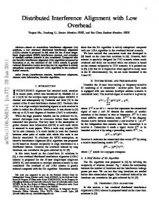
B. Backhaul overhead Considering the different IA-Cell assignment schemes, their required backhaul overhead (excluding the feedback overhead) are summarized in Table II, where ”One-sided”/”Twosided”/”Centralized”/”Fixed” denotes the IA-Cell assignment by the one-sided/two-sided/centralized/fixed matching. During the IA-Cell assignment by the one/two-sided matching, if BS k ′ asks, definitely accepts, temporarily accepts or definitely rejects BS k, it will send ”01”, ”11”, ”10” or ”00” to BS k, respectively, each of which can be conveyed into a QPSK symbol. In particular, the one-sided matching by the FCA takes K + (NC − 1) steps where NC denotes the number of cycle chains, and each step has one ask. The two-sided matching by the Basic Gale-Shapley algorithm [36] takes [K, K(K − 1) + 1] proposals. After assignment by the one-sided matching, each cell needs to send an explicit inner precoder to its corresponding IA-provider, while it is not necessary for the two-sided matching because it has been already exchanged before assignment. After the quantization of the precoder patterns, each BS needs to exchange the corresponding indexes with others, based on which the new ZF decoder can be designed. The resulting total backhaul overhead is reported in Table II. C. Complexity As shown in Section III, the complexity of computing K IA precoders by the GIA is KO((L − 1)2 LNB2 NU ). For the one-sided matching, the complexity mainly depends on the preference generation as in (19). The generation of K ranked preference lists takes K(K − 1)L(O(NB NU ds ) + 2L(O(NU NB2 ) + O(NU3 )) + 2O(NB d2s ) + 2O(d3s ) + KO(K)) arithmetic operations. The FCA with K + (NC − 1) steps has the complexity O(K) where NC denotes the number of cycle chains. For the two-sided matching, besides generating (19), K ranked preference lists generation as in (20)
requires K(K −1)L O(2NU2 ds ) + O(NU NB ds ) + 2(O(d3s ) + KO(K) arithmetic operations. The complexity of the Basic Gale-Shapley algorithm with at most K 2 − K + 1 steps is upper bounded by O(K 2 ). The centralized assignment needs k PK to compute K! k=0 (−1) possible rate performance with k! PK (−1)k the complexity K! k=0 k! K(L(O(2NU2 ds )+O(NB2 ds )+ (L + 1)O(NB NU ds ) + (L + 2)O(d3s ) + (L + 2)O(NB d2s ))). Roughly speaking, the one-sided matching, the two-sided matching and the centralized assignment mainly take K(K − P (−1)k 1)L, 2K(K − 1)L and K! K ”rate-like” computak=0 k! tions9 , respectively. Fig. 1 shows the gross complexity of these three algorithms over the number of cells. It implies the centralized assignment is a reasonable approach with a comparable complexity as the distributed algorithms if K ≤ 4. 9 The computation expression is not the actual rate expression, but always H has the form log det(I + XΠ⊥ Y X ).

500 No. of "Rate" Computations

•

400

Centralized Two−sided One−sided

300

200

100

0 3

4 No. of Cells

5

Fig. 1: Complexity comparison of the stable matching and centralized assignment

Instead, when K ≥ 5 distributed algorithms are preferable from the perspective of complexity. VII. N UMERICAL R ESULTS In this section, the performance of the GIA with optimized IA-Cell assignment under both the unlimited and limited feedback is evaluated. A. System Model and Performance Metrics We consider a (K, L, NB , NU , ds ) = (4, 2, 14, 8, 2) interfering MIMO-MAC. We set σk2 = 1, ∀k and Pi,k = P, ∀i, k, respectively. Let SN R = 10 log10 (P ) denote the transmit signal-noise ratio (SNR).The path loss of direct links and cross links are set to be 1, and to satisfy randomly and uniformly distribution in [0, 1], respectively.10 To properly measure the performance of the proposed approaches, we consider two following metrics K X L   X bi,k , Rmin , E R Rsum , E k=1 i=1

min

k=1,...,K

L X i=1

 bi,k , R

bi,k is given in (41). Rsum and Rmin are the average where R sum-cluster rate and the average minimum single-cell rate over different channel realizations to measure the overall cluster throughput and the fairness of the cluster, respectively. B. Performance Comparison with Perfect Feedback Under unlimited feedback, the effect of IA-Cell assignment on Rsum and Rmin is evaluated by the following metrics. • Uppersum and Lowersum (Uppermin and Lowermin) denote the performance achieved by the best and the worst IA-Cell assignment for sum cluster-rate maximization (minimum cluster-rate maximization), respectively, which are determined by the centralized assignment; • Two/One/Fixed: Each channel realization is under the IA-Cell assignment by the two-sided/one-sided/fixed matching (6); 10 This is to guarantee that interference channels are not stronger than direct channels, since a user is usually assigned to the BS who provides it the strongest link. The user selection and user-BS association can be done based on the uplink CSI available at BSs, which is out of the scope of this work.

11

TABLE II: Total backhaul overhead of K cells Algorithms One-sided Two-sided Centralized Fixed

Before assignment 0 K(K − 1)LNU ds cc (K−1)2 LNU ds + cc (K−1)LNU NB 0

Assignment 4(K + (NC − 1)) bit 4[K, K 2 − K + 1] bit 0 –

After assignment KLNU ds cc +(K − 1)B bit (K − 1)B bit (K − 1)LNU ds cc +(K − 1)B bit KLNU ds cc

1) ”cc” denotes the unit of a complex coefficient. 2) Each ask is responsed during the assignment.

120

70 Uppersum

Uppersum Two One Fixed RB FDMA

[bpcu]

60

60

sum

sum

80

Lower

R

Rsum [bpcu]

100

40

5

10

15 SNR [dB]

20

25

500

120 bit

min

min

12

min

[bpcu]

Two One Fixed RB FDMA

R

[bpcu] min

R

Upper

Lower

5

0 0

200 300 400 Sum feedback bit budget [bit]

14

Uppermin

10

40 bit

Fig. 4: Sum-cluster rate comparison under limited feedback w.r.t. SNR.

25

15

40

20 100

30

Fig. 2: Sum-cluster rate comparison under unlimited feedback w.r.t. SNR.

20

50

30

20 0 0

80 bit

Two One Fixed

Two One Fixed

10

8

80 bit

6

5

10

15 SNR [dB]

20

25

30

Fig. 3: Minimum single-cell rate comparison under unlimited feedback w.r.t. SNR. → − RB: Each precoder V i,k is a random subspace and each decoder is the ”matched filter” U i,k = k,H k − 21 ; H ki,k V i,k (V H i,k H i,k H i,k V i,k ) • FDMA: Each user ocuppies an un-overlapped spectrum. Both Fig. 2 and Fig. 3 show that a large performance gap exists between the best IA-Cell assignment and the worst IA-Cell assignment. It implies the IA-Cell assignment has a significant influence on both the overall throughput and the fairness. E.g., this performance gap regarding Rsum is as large as 5 dB and that of Rmin is even larger than 10 dB for high SNR. Compared with the fixed matching, the two-sided and one-sided matching have a similar performance improvement, i.e., more than 1 dB for Rsum and more than 5 dB for Rmin . The advantage of the GIA is significant compared with the random beamforming and FDMA, especially for high SNR. •

C. Performance Comparison under Limited Feedback Under limited feedback, the proposed DBA is evaluated by comparing with the classical EBA (plotted in dashed lines in the following figures). The random subspace codebook is adopted in the quantization.

4 100

200 300 400 Sum feedback bit budget [bit]

500

Fig. 5: Minimum single-cell rate comparison under limited feedback w.r.t. SNR.

1) Performance comparison w.r.t. feedback bit: The performance w.r.t. the sum feedback bit budget is evaluated when SN R = 25 dB. Fig. 4 shows that the sum-cluster rate is increasing with the sum feedback bit budget and at an approximate linear rate – around 0.09, which coincides with 1 ds (NU −ds ) = 0.0833 in (44). The proposed DBA outperforms the EBA in both the sum cluster-rate in Fig. 4 and the minimum single-cell rate in Fig. 5. Compared with the fixed matching with the EBA, the proposed centralized assignment and the distributed stable matching with the DBA can save around 80 bit and 40 bit, respectively, to achieve Rsum = 50 bpcu in Fig. 4, and around 120 bit and 80 bit, respectively, to achieve Rmin P = 10k bpcu in Fig. 5. The sum-cluster RINR in 10 log10 ( K ℓ=1 Iℓ ) dB is linearly decreasing with sum feedback bit budget as shown in Fig. 6. The DBA achieves a lower RINR compared with the EBA, which implies that the effectiveness of minimizing the upper bound of sum-cluster RINR in (28). The sum-cluster RINR is greatly larger than ds in Fig. 6, making the approximation in (43) feasible. 2) Performance comparison w.r.t. SNR: The proposed algorithms are evaluated by measuring the sum-cluster rate and

12

34

15 Uppermin

Two One data4

Two One Fixed

26

[bpcu]

24

R

30 28

10

500 bit

min

Sum RINR [dB]

Upper

sum

32

5

22

300 bit

20 18 100

200 300 400 Sum feedback bit budget [bit]

0 0

500

Fig. 6: Sum-cluster RINR comparison under limited feedback w.r.t. SNR.

5

Upper

P ROOF

25

30

A PPENDIX A OF P ROPSOSITION 3 IA

30

Ik ,

300 bits

20

K X

k Im = Iℓk

(50a)

m=1,m6=k

10 0 1

20

Proof: Considering Cell ℓ −→ Cell k, we have

40

R

sum

[bpcu]

50

500 bits

sum

Two One Fixed

15 SNR [dB]

Fig. 8: Minimum single-cell rate comparison under limited feedback w.r.t. SNR.

70 60

10

2

3

4 SNR [dB]

5

6

7

Fig. 7: Sum cluster-rate comparison under limited feedback w.r.t. SNR. the single-cell rate performance w.r.t. SNR for the fixed sum feedback budget B = 300 bit and B = 500 bit, respectively. From Fig. 7 and Fig. 8, it is observed that the performance with B = 500 bits is much greater than that with B = 300 bits and the performance gap enlarges with the SNR. E.g., for SN R = 30 dB, the gap of sum-cluster rate and that of the single-cell rate are as large as around 20 bpcu and 8 bpcu, respectively. From the perspective of energy consumption, the feedback of B = 500 bits results in a higher complexity and more feedback energy consumption than the feedback of B = 300 bits, while it is still attractive when the battery power saving is focused, because user terminals are usually powered by battery and BSs are powered by electric networks, and the more scarce battery energy can be saved at the cost of the BS energy. E.g., 15 dB uplink power can be saved by the stable matching to achieve Rsum = 40 bpcu with B = 500 bits compared with B = 300 bits. Compared to the fixed matching with EBA, the proposed centralized assignment and stable matching with DBA can reduce by 10 dB and 5 dB uplink power, respectively, to achieve Rsum = 60 bpcu. And this performance improvement enlarges with SNR. VIII. C ONCULSIONS In this work, we provide a framework for the GIA with optimized IA-Cell assignment in the interfering MIMO MAC network under limited feedback. This algorithm yields the closed-form IA transceiver by distributed implementation at BS side if its feasible conditions are satisfied. Furthermore, the effect of IA-Cell assignment and DBA on either the sumcluster rate or minimum single-cell rate are discussed and illustrated in the simulations.

≤

L   H X Pi,ℓ b H k,H Π⊥ k in H k Vb i,ℓ V Tr i,ℓ i,ℓ i,ℓ H 1,ℓ V 1,ℓ σ2 d i=1 k s

(50b)

L X Pi,ℓ H k = 2 d Tr(S i,ℓ Ωi,ℓ S i,ℓ Σi,ℓ ) σ i=1 k s

(50c)

≤

(50d)

ds L X Pi,ℓ X λd (Ωki,ℓ )βi,d 2d σ s k i=1 d=1

ds L X X Pi,ℓ k ≤ λ1 (Ωi,ℓ ) βi,d σ2 d i=1 k s

(50e)

=

(50f)

d=1

L X → − Pi,ℓ λ1 (Ωki,ℓ )d2c (Vb i,ℓ , V i,ℓ ) 2 σ d i=1 k s

≤ c(NU , ds )

L B X Pi,ℓ − ds(N i,ℓ k U −ds ) , λ (Ω )2 1 i,ℓ 2d σ s k i=1

(50g)

where (50b) is derived based on the inequality of ⊥ 2 2 ||Π⊥ [Y 1 ,Y 2 ] Y 3 ||F ≤ ||Π[Y 1 ] Y 3 ||F . Plugging (24) into (50b) and removing the zero-valued terms and based on the definition (29) yield (50c), where S i,ℓ ∈ CNU ×ds satisfies SH i,ℓ S i,ℓ = I ds and Σi,ℓ = diag{βi,1 , . . . , βi,ds }, ∀i is with P s → − βi,d ∈ [0, 1], ∀d and dd=1 βi,d = d2c (Vb i,ℓ , V i,ℓ ). The upper bound (50d) is achieved when the truncated unitary matrix S i,ℓ is the eigen-subspace of the matrix Ωki,ℓ associated with the ds largest eigenvalues λ1 (Ωki,ℓ ), . . . , λds (Ωki,ℓ ). (50g) is derived by the quantization distortion upper bound (25). A PPENDIX B P ROOF OF L EMMA 2 Proof: The quantization Vb can be exactly expressed by the N -dimensional full space V ∪ V ⊥ as ⊥ b Vb = ΠV Vb + Π⊥ V V = V C 1 + V C 2,

(51)

where C 1 ∈ CN ×N and C 2 ∈ C(M−N )×N in (51) denote the components of Vb projected on the V and V ⊥ , respectively.

13

From (51), it is derived the properties of C 1 and C 2 as H

H Vb Vb = I N ⇒ C H 1 C1 + C2 C2 = IN ;

(52)

H

d2c (Vb , V ) = N − Tr(Vb Vb V V H ) ⇒

2 b Tr(C 2 C H 2 ) = dc (V , V ).

(53)

By the singular-value decomposition (SVD), C 1 is ex1/2 H eigenvalues ΛC 1 , pressed n by C 1 = U C 1 ΛC 1 V C 1 where o

H diag λ1 (C H satisfy λn (C H 1 C 1 ), . . . , λN (C 1 C 1 ) 1 C 1) ≥ PN H 0, ∀n subject to n=1 λn (C 1 C 1 ) = N − d2c (Vb , V ) based on (52) and (53). From (52), we further derive C H 2 C2 = H  0 , which requires λ (C V C 1 (I N − ΛC 1 )V H N n 1 C 1) ≤ C1 1, ∀n. Therefore, C 2 can be expressed by

e (I N − ΛC )1/2 V H C2 = U 1 C1

(54)

e ∈ C(M−N )×N satisfying U e HU e = I N is to select where U a N -dimensional subspace from the M − N -dimensional null space Span{V ⊥ }. R EFERENCES [1] J. G. Andrews, S. Buzzi, W. Choi, S. Hanly, A. Lozano, A. C. K. Soong, and J. C. Zhang, “What will 5G be?,” IEEE J. Sel. Area. Comm., 2014, to appear: available at http://arxiv.org/abs/1405.2957. [2] D. Gesbert, S. Hanly, H. Huang, S. Shamai, O. Simeone, and W. Yu, “Multi-cell MIMO cooperative networks: A new look at interference,” IEEE J. Sel. Area. Comm., vol. 28, no. 9, pp. 1–29, Dec. 2010. [3] 3GPP TR36.913 V2.0.1, “Evolved Universal Terrestrial Radio Access (E-UTRA); Further advancements for E-UTRA Physical layer aspects,” Mar. 2010. [4] R. Irmer, H. Droste, P. Marsch, and et al., “Coordinated multipoint: Concepts, performance, and field trial results,” IEEE Commun. Mag., pp. 102–111, Feb. 2011. [5] J. Kim, S. H. Park, H. Sung, and I. Lee, “Sum rate analysis of two-cell MIMO broadcast channels: Spatial multiplexing gain,” in Proc. of IEEE ICC, 2010. [6] S. A. Jafar, “Interference alignment-A new look at signal dimensions in a communication network,” Found. and Trends in Commun. and Inf. Theory, vol. 7, no. 1, pp. 1–134, 2011. [7] V. R. Cadambe and S. A. Jafar, “Interference alignment and degrees of freedom of the K-user interference channel,” IEEE Trans. Inf. Theory, vol. 54, no. 5, pp. 3425–3441, Aug. 2008. [8] S. W. Choi, S. A. Jafar, and S.-Y. Chung, “On the beamforming design for efficient interference alignment,” IEEE Commun. Lett., vol. 13, no. 11, pp. 847–849, Nov. 2009. [9] H. Sung, S.-H. Park, K.-J. Lee, and I. Lee, “Linear precoder designs for K-user interference channels,” IEEE Trans. Wirel. Commun., vol. 9, no. 1, pp. 291–301, Jan. 2010. [10] I. Santamaria, O. Gonzalez, R. W. Heath Jr., and S. W. Peters, “Maximum sum-rate interference alignment algorithms for MIMO channels,” in Proc. IEEE GLOBECOM, Dec 2010. [11] K. S. Gomadam, V. R. Cadambe, and S. A. Jafar, “A distributed numerical approach to interference alignment and applications to wireless interference networks,” IEEE Trans. Inf. Theory, vol. 57, no. 6, pp. 3309–3322, Jun. 2011. [12] V. Nagarajan and B. Ramamurthi, “Distributed cooperative precoder selection for interference alignment,” IEEE Trans. Veh. Technol., vol. 59, no. 9, pp. 4368–4376, Nov. 2010. [13] C. Suh, M. Ho, and D. N. C. Tse, “Downlink interference alignment,” IEEE Trans. Commun., vol. 59, no. 9, pp. 2616–2626, Sep. 2011. [14] C. M. Yetis, T. Gou, S. A. Jafar, and A. H. Kayran, “Feasibility conditions for interference alignment,” IEEE Trans. Signal Process., vol. 58, pp. 4771–4782, Sep. 2010. [15] T.Kim, D. J. Love, B. Clerckx, and D. Hwang, “Spatial degrees of freedom of the multi-cell multiple access channel,” in Proc. IEEE Globecom, 2011.

[16] W. Shin, N. Lee, J-B. Lim, C-Y. Shin, and K. Jang, “On the design of interference alignment scheme for two-cell MIMO interfering broadcast channels,” IEEE Trans. Wirel. Commun., vol. 10, no. 2, pp. 437–442, Feb. 2011. [17] J. Tang and S. Lambotharan, “Interference alignment techniques for MIMO multi-cell interfering broadcast channels,” IEEE Trans. Commun., vol. 61, no. 1, pp. 4907–4922, Jan. 2013. [18] E. Dahlman, S. Parkvall, and J. Skoeld, 4G: LTE/LTE-Advanced for mobile broadband, May 2011. [19] D. J. Love, R. W. Heath Jr., V. Lau, D. Gesbert, B. D. Rao, and M. Andrews, “An overview of limited feedback in wireless communication systems,” IEEE J. Sel. Area. Comm., vol. 26, no. 8, pp. 1341–1365, Oct. 2008. [20] N. Jindal, “MIMO broadcast channels with finite-rate feedback,” IEEE Trans. Inf. Theory, vol. 52, no. 11, pp. 5045–5060, Nov. 2006. [21] T. Yoo, N. Jindal, and A. Goldsmith, “Multi-antenna downlink channels with limited feedback and user selection,” IEEE J. Sel. Area. Comm., vol. 25, no. 11, pp. 1478–1491, Sep. 2007. [22] N. Ravindran and N. Jindal, “Limited feedback-based block diagonalization for the MIMO broadcast channel,” IEEE J. Sel. Area. Comm., vol. 26, no. 8, pp. 1473–1482, Oct. 2008. [23] S. Schwarz and M. Rupp, “Subspace quantization based combining for limited feedback block-diagonalization,” IEEE Trans. Wirel. Commun., vol. 12, no. 11, pp. 5868–5879, Nov. 2013. [24] X. Rao, L. Ruan, and V. Lau, “Limited feedback design for interference alignment on MIMO interference networks with heterogeneous path loss and spatial correlations,” IEEE Trans. Signal Process., vol. 61, no. 10, pp. 2598–2607, May 2013. [25] H. Bolsckei and I. Thukral, “Interference alignment with limited feedback,” in Proc. of IEEE ISIT, Jul. 2009. [26] R. T. Krishnamachari and M. K. Varanasi, “Interference alignment under limited feedback for MIMO interference channels,” in Proc. IEEE ISIT, Jun. 2010. [27] M. Rezaee and M. Guillaud, “Interference alignment with quantized Grassmannian feedback in the K-user constant MIMO interference channel,” 2012, submitted to IEEE Trans. Inf. Theory: available at http://arxiv.org/abs/1207.6902. [28] M. Alodeh, S. Chatzinotas, and B. Ottersten, “Spatial DCT-based channel estimation in multi-antenna multi-cell interference channels,” 2014, submitted: available at http://arxiv.org/abs/1401.6690. [29] G. Gupta and A. K. Chaturvedi, “User selection in MIMO interfering broadcast channels,” 2013, submitted to IEEE Trans. Commun.: available at http://arxiv.org/abs/1310.7425. [30] “3D Computer Vision Script Draft,” TU Munich Leture: available at http://campar.in.tum.de/Chair/TeachingWs05ComputerVision. [31] M. Hassani, “Derangements and applications,” J. Integer Seq., vol. 6, pp. 1–8, 2003. [32] Y. Yuan, “Residence exchange wanted: A stable residence exchange problem,” Eur. J. of Oper. Res., vol. 90, no. 3, pp. 536–546, May 1996. [33] L. Shapley and H. Scarf, “On cores and indivisibility,” J. Math. Econ., vol. 1, no. 1, pp. 23–37, Mar. 1974. [34] P. Biro, D. F. Manlove, and S. Mittal, “Size versus stability in the marriage problem,” Theoretical Computer Science, pp. 1828–1841, 2010. [35] D. Gusfield and R. Irving, The Stable Marriage Problem: Structure and Algorithms, MIT Press, Cambridge, Massachusetts, 1989. [36] D. Gale and L. Shapley, “College admission and the stability of marriage,” Amer. Math. Monthly, vol. 69, no. 1, pp. 9–15, Jan. 1962. [37] D. J. Love and R. W. Heath Jr., “Limited feedback unitary precoding for spatial multiplexing systems,” IEEE Trans. Inf. Theory, vol. 51, no. 8, pp. 2967–2976, Aug. 2005. [38] A. Ashikhmin and R. Gopalan, “Grassmannian packings for efficient quantization in MIMO broadcast systems,” in Proc. of IEEE ISIT, 2007. [39] K. Schober, P. Janis, and R. Wichman, “Geodesical codebook design for precoded MIMO systems,” IEEE Trans. Inf. Theory, vol. 13, no. 10, pp. 773–775, Aug. 2009. [40] A. Medra and T. N. Davidson, “Flexible codebook design for limited feedback systems via sequential smooth optimization on the Grassmannian manifold,” IEEE Trans. Signal Process., vol. 62, no. 5, pp. 1305– 1318, Mar. 2014. [41] W. Dai, Y. Liu, and B. Rider, “Quantization bounds on Grassmann manifolds and applications to MIMO communications,” IEEE Trans. Inf. Theory, vol. 54, no. 3, pp. 1108–1123, Mar. 2008. [42] C. Sun and E. A. Jorswieck, “Low complexity sum rate maximization for single and multiple stream MIMO AF relay networks,” 2012, available at http://arxiv.org/abs/1211.5884.