Noname manuscript No. (will be inserted by the editor)
GRowing Algorithm for Intersection Detection (GRAID) in branching patterns Joan M. N´ un ˜ ez · Jorge Bernal · F. Javier S´ anchez · Fernando Vilari˜ no
Received: date / Accepted: date
Abstract Analysis of branching structures represents a very important task in fields such as medical diagnosis, road detection or biometrics. Detecting intersection landmarks becomes crucial when capturing the structure of a branching pattern. We present a very simple geometrical model to describe intersections in branching structures based on two conditions: Bounded Tangency condition (BT) and Shortest Branch (SB) condition. The proposed model precisely sets a geometrical characterization of intersections and allows us to introduce a new unsupervised operator for intersection extraction. We propose an implementation that handles the consequences of digital domain operation that, unlike existing approaches, is not restricted to a particular scale and does not require the computation of the thinned pattern. The new proposal, as well as other existing approaches in the bibliography, are evaluated in a common framework for the first time. The performance analysis is based on two manually segmented image data sets: DRIVE retinal image database and COLON-VESSEL data set, a newly created data set of vascular content in colonoscopy frames. We have created an intersection landmark ground truth for each J.M. N´ un ˜ez (B) · J. Bernal · F.J. S´ anchez · F. Vilari˜ no Computer Vision Centre and Computer Science Department, Campus Universitat Aut` onoma de Barcelona, 08193 Bellaterra, Barcelona, Spain Tel.: +34 935 811 828 Fax: +34 935 811 670 E-mail:
[email protected] J. Bernal E-mail:
[email protected] F.J. S´ anchez E-mail:
[email protected] F. Vilari˜ no E-mail:
[email protected]
data set besides comparing our method in the only existing ground truth. Quantitative results confirm that we are able to outperform state-of-the-art performance levels with the advantage that neither training nor parameter tuning is needed. Keywords Bifurcation · Crossroad · Intersection · Retina · Vessel
1 Introduction Branching structures are common in nature. Patterns such as vascular trees, road networks, palm prints or topographical structures like rivers are just some examples. The detection of these structures, their characterization and the measurement of the network properties are crucial tasks for subsequent applications. These networks are piecewise elongated structures that cross over each other or branch off more or less frequently. Branching points become important landmarks for any application that intends to characterize the original pattern. Intersection landmark extraction has been mentioned and studied in several fields in the last decades. The presence of branching structures in medicine and biology has been widely reported [2,22]. Retinal blood vessel morphology has been described as an important indicator of hypertension, diabetes, arteriosclerosis or other cardiovascular diseases [14,26]. Retinal vascular trees or palm prints have also been reported as reliable biometrics for personal identification tasks [21] or registration systems [12]. Vascular structures have also recently been claimed to be of relevance in the analysis of colonoscopy scenes. Blood vessels are a source of information of intensity valleys and the correct identification of blood vesselsrelated valleys has been proven to lead to an improve-
2
ment of the state-of-the-art methods in polyp localization [7,6,18]. An accurate identification or segmentation of blood vessels could be of use, for instance, to unequivocally identify regions of the colon surface by tracking ramifications of vascular structures. In this paper, we propose a method to extract branching landmarks -i.e., intersections- from any kind of network pattern. Although our proposal is applied here in the context of medical 2D structures, it is straightforward generalisable to 3D or any kind of branching pattern. We provide performance results on the DRIVE public retinal image data set [24] using the public intersection landmark ground truth defined in [4]. We also contribute with: 1) a novel intersection ground truth for the same DRIVE data set, and 2) the only existing up to date colonoscopy data set which includes manually segmented images from colonoscopy videos and its corresponding intersection landmark ground truth vessel patterns. The remaining sections are organized as follows: in Section 2 we introduce previous approaches to vessel landmark extraction. In Section 3 we present our intersection characterization model and how it leads to a simple and accurate landmark detector. Section 4 presents our experiments for intersection detection. Section 5 includes the analysis of qualitative and quantitative results based on DRIVE and novel COLONVESSEL data sets. Main conclusions are exposed in Section 6.
Joan M. N´ un ˜ez et al.
(a)
(b)
Fig. 1 Usual thinning artifacts. (a) Original patterns. (b) Thinning results with artifacts (Necking: green, Tailing: red, Spurs: orange).
vascular trees. A skeleton, which has not a unified definition for the different implementations, is generated by a process of thinning. This process starts from the original structure and must identify the pixels belonging to it that are essential to keep the original structure shape [19]. Skeletonized shapes are usually affected by thinning artifacts like necking, tailing, spurs or staircase artifacts (see Figure 1), which landmark detectors will have to handle [19]. Martinez-Perez et al. [20] proposed a characterization of retinal vascular content based on the one-pixel wide tree computed from the vessel pattern. Skeleton pixels are scanned in a 3 × 3 neighborhood so that bifurcation and crossover candidates are extracted by selecting skeleton pixels with 3 or 4 neighbors respectively. They propose a semiautomatic method to overcome the fact that close bifurcations are usually joint into a crossover. Chanwimaluang et al. [13] proposal performs a similar first candidate selection procedure followed by a second processing step that removes small intersections by using the boundary pixels of an 11 × 11 window. Jung et al. [16] detector of vascular landmarks 2 Related work is also use the skeleton to detect crossroads as cross perpendicular structures with four connections and biThe existing approaches for vascular intersection defurcations as Y-type structures. tection, fundamentally proposed in the field of retinal imaging, can be separated into three categories [4,9]: Bhuiyan et al. [9] method extracts vascular landmarks from the centerline image by using 3 × 3 rotageometrical-feature based methods and model based methods. tional invariant masks to select potential candidates. The candidates are analyzed to find geometrical and topological properties that are used to classify landmark candidates as bifurcations or crossovers. Ardiz2.1 Geometrical-feature based methods zone et al. work [3] included vascular landmark extraction again based on the connectivity of the one-pixel Geometrical-feature based approaches usually perform wide vascular tree without any further candidate seleca pixel-level processing stage followed by different kinds tion. of post-processing analysis. These approaches usually involve adaptive filtering and branch analysis based on Another approach called combined cross-point numthinned structures. They are often computationally costly ber (CNN) method is introduced in [1]. This is a hysince they involve the processing of each pixel indepenbrid method of two intersection detection techniques: dently. An important step of the methods in this catthe simple cross-point number (SCN) [8] and the modiegory usually consists of a thinning algorithm leading fied cross-point number (MCN) method. The former is to compute the so-called skeleton of the structure (as based on a 3 × 3 window that is placed in the considin [9,13,16,20]. These methods claim that it is desirered pixel to compute its so-called cross-point number able to reduce the original structures to one-pixel wide (cpn), which basically counts the number of converging
GRowing Algorithm for Intersection Detection (GRAID) in branching patterns
branches to the pixel. Bifurcation points must hold 3 transitions (cpn = 3). This method follows the same idea as the previous approaches. However, the authors propose a solution to the problem of turning a crossroad into a pair of bifurcations. The solution is based on MCN, a new operator based on a 5 × 5 which also computes the number of converging branches to the pixel but, in this case, in a 5-side window parameter. The work proposed by Calvo et al. [10] also reduces the vascular structure to its skeleton, which is filtered to reduce spurious projections. The skeleton pixels are then classified by using their intersection number, equivalent to the already mentioned SCN, followed by post-processing techniques to solve crossover detection problems based on the intersections between a circumference of a given radius and the thinned pattern tree. The authors propose a voting system which involves three different radii. Finally, the classification is refined by merging two bifurcations into a crossroad if they are close enough (represented by a radius parameter) and connected by a single segment. Saha et al. [23] method also takes skeleton tree extracted from the vascular structure and does not detect crossroads. They consider a window centered in the candidate pixel and each connected-component is uniquely labelled. The algorithm makes an anti-clockwise roundtrip along the perimeter of the window. A pixel is classified as a bifurcation point if the cyclic path length is 3 and does not have any repetition. 2.2 Model based methods These group of methods is based on a vectorial tracing of the desired structure. Seed points are usually placed as initial locations so that the vascular structures in the image can be tracked from them recursively. These methods usually have lower computational complexity than the methods in the previous category as they do not need to process every pixel in the image so they are usually proposed for real-time applications. The method introduced by Can et al. [11] is based on an antiparallel edges model of the linear portions of the vascular pattern. The algorithm keeps relevant tracing information in two data structures as the tracking of the branching pattern proceeds, the so-called ”centerline image” and ”centerline network”. The former is an array which keeps non-zero values for the already traced centerlines and increments a variable called the ”segment number” when each new segment in the vascular structure is tracked. The latter consists of a linked list of segments so that every single segment is a linked list of connected pixels which represent the already traced centerline of that segment. The centerline
3
image is checked from the current tracing point to label it as a bifurcation candidate if non-zero values are found in three different small line searches. At the same time, the centerline network is searched every time a previously detected vessel is intersected and the intersection point is updated. When multiple close intersections are detected they are replaced by their centroid. Tsai et al. [25] presented an exploratory or tracking approach named exclusion region and position refinement (ERPR). This approach is also based on the antiparallel model. Nevertheless, this work considers this model is valuable for the tracing algorithm itself but it is no longer valid when approaching intersection or branching points. As a consequence, the authors claim that the estimation of vascular landmarks is clearly affected. They propose a model for intersections based on the landmark location, the set of vessel orientations that meet in the intersection and a circular exclusion region where the antiparallel model is violated. The landmark extraction algorithm starts at an endpoint of the trace, either when it intersects another vessel or when it meets at least two other trace endpoints. They launch an iterative process from those endpoints that re-estimates the traces when outside exclusion regions and re-estimates the landmark position otherwise. 2.3 Hybrid approaches Azzopardi et al. [4] introduced a different approach proposing the use of so-called COSFIRE (Combination Of Shifted FIlter REsponses) filters [5]. COSFIRE filters are keypoint detection operators that must be trained to extract given local patterns. These filters are made up of Gabor filters that are combined so that the response of a given pixel is computed as a combination of the shifted responses of the Gabor filters. The final output includes the local maxima from the outputs of all trained filters. In this paper we introduce our GRowing Algorithm for Intersection Detection (GRAID), which is a hybrid approach based on the definition of a precise intersection model that operates at pixel level. The intersection model allows us to define the landmark which represents the location of an intersection. The model is defined by two conditions: Bounded Tangency (BT) condition, and Shortest Branch (SB) condition. The algorithmic implementation has one single parameter that states the leverage between the geometrical proportions of the branches and the intersection. The method is not restricted to the computation of the thinned pattern nor conditioned by a sliding window size. For these reasons the algorithm is independent from drawbacks of thinning methods and it is not restricted to any particular
4
Joan M. N´ un ˜ez et al.
(a)
(b)
(c)
Fig. 2 Intersection model: candidate examples. (a) Positive (verifies both BT and SB conditions). (b) Negative (does not verify BT condition). (c) Negative (verifies BT condition but does not verify SB condition).
scale. The outcome is a straightforward and precise intersection detector which does not need to go through a training process and that is able to classify separately the intersections regarding its number of branches.
3 Methodology We propose a method to extract bifurcations and crossroads from branching patterns in binary images based on a general intersection model. A precise model to allow the definition of the landmarks representing the location of intersections is stated. Given that model, an algorithm which handles the consequences of working on a digital domain, such as the approximation of the Euclidian distance and the lack of resolution to reach maximal ball tangencies, is proposed. The first part of this section introduces our proposed model and the second part proposes the corresponding implementation of the detector.
3.1 Intersection model An intersection candidate is defined by the center of a maximal circumference inscribed in the branching pattern. The candidates are extracted as intersections if and only if they hold the following two conditions: – Bounded Tangency (BT): the maximal inscribed circumference and the pattern contour must have 3 or more tangencies. – Shortest Branch (SB): the relation between the shortest branch and the radius of the inscribed circumference must be higher than a given ratio. Given a binary image containing a structure pattern, S, and a point, x ∈ S, we define the circumferences with a radius r, centered at x and inscribed in S as CS (x, r), where 0 < r ≤ rmax . When r = rmax the circumference is maximally circumscribed. Then, a
decision function for intersection extraction is defined as follows: B(x) = |PS ∩ CS (x, rmax )|
(1)
where PS is the contour of the structure, S. The verification of BT condition is achieved through the analysis of B(x) function. B(x) describes the number of tangent points between the maximal inscribed circumference and the branch pattern contour. Every single point within S will be forwarded as an intersection candidate if the number of tangent points between the inscribed circumference and the structure contour is ≥ 3. Since the number of tangencies is equivalent to the number of branches, B(x) also describes the number of branches converging at each intersection candidate. Regarding the usual terminology in the bibliography, those points verifying B(x) = 3 will be bifurcation candidates (3 branches) and those verifying B(x) = 4 will be crossroad candidates (4 branches). Our model allows in this way to separately extract intersections with a particular number of branches, although we will focus in this work in general intersection extraction by simply allowing B(x) ≥ 3. After verifying BT condition each branch must be tracked to assess that SB condition imposed by our model is also held. SB condition is mathematically defined as: rmax max{rmax − Cost(n)}, ∀n n
(5)
2. The difference between the maximum radius from each neighbor and the distance to that neighbor is positive, and the maximal ball radius from the candidate pixel is higher than the minimum cost to reach a neighbor: n {rmax − Cost(n) > 0} ∨ {rmax > min{Cost(n)}}, ∀n(6) n
Algorithm 1: Algorithm Input: image: Input binary image, δ: minimum branching factor Output: output: Intersection binary image dM ap = DanielssonDistance(Cost,!image); for pix in image do if IsBallCenter(pix,dM ap) then f rontier = ExpandCenter(pix,dM ap,Cost); len = dM ap(pix)*δ; nbranch = ExpandFrontier(f rontier,Cost,len); if nbranch > 2 then output(pix) = true; end end end return output;
The inequality in 1) would be enough if the Euclidean distance was properly defined in a discrete domain. The approximation with the Cost function forces the introduction of the or-condition in 2). Figure 4b shows an example of maximal ball centers by IsBallCenter. Every ball center is then analysed further so that the second part of BD condition is tested. We must select those maximal ball centers which have at least 3 tangencies to the pattern contour, i.e. at least 3 branches. To asses the number of branches we must expand the ball from its center to its radius. This task is achieved by ExpandCenter function (line 4). The discrete domain can cause the maximal circumference radii we already computed to be too short to reach all the expected tangent points. We handle this problem by adding an offset
6
Joan M. N´ un ˜ez et al.
(a)
(b)
(c)
(d)
(e)
Fig. 4 Algorithm samples. (a) Intersection pattern. (b) Maximal ball candidates. (c) Maximal ball (green) and 2 outer branch frontiers (orange). (d) Extended maximal ball (green) and 3 outer branch frontiers (orange). (e) Frontier expansion (blue)
equivalent to the maximum value of the Cost function to the radius of the maximal ball:
r′max = rmax + max{Cost(n)} n
(7)
With this offset we make sure that the algorithm reaches the contour and the right amount of tangencies are identified. This improvement saves us from missing maximal ball centers with 3 or more branches (see Figure 4c and 4d for an example). ExpandCenter function (line 4) expands every center pixel to its maximal ball contour. The pixels that are part of that contour are tested to isolate those that have at least one neighbor that is part of the structure (foreground) and out of the maximal ball. Those isolated pixels are then grouped in connected blobs that we call branch frontiers (see Figure 4d). Finally, branch frontiers need to be expanded as shown by Figure 4e (line 6) to assess the verification of SB condition. The corresponding ball center pixel will be labelled as an intersection candidate if and only if at least 3 branches verify SB condition expressed by Equation 2 (line 7). Algorithm 2 shows the explicit pseudocode implementation of ExpandCenter and ExpandFrontier. The algorithm expands a given pixel based on the distance map by prioritizing the expansion of those pixels with a lower distance cost until the corresponding StopCondition is reached (line 17). In the case of ExpandCenter, the stop condition is to reach a frontier pixel. In the case of ExpandFrontier the condition would consist of reaching the branch distances that assess SB condition (Equation 2). The final output of the algorithm are the centroids of the landmark candidate blobs since several candidates may be selected for a given intersection due to the discrete working domain.
Algorithm 2: Expand Input: pix: pixel to be expanded dM ap: Danielsson Distance map to background CostF unc: 8 connectivity cost function Output: output: number of frontiers/branches Make-Queue: queue; queue.P ush(pix); Cost = ascendingSort(CostF unc); temp = dM ap; while !queue.isEmpty do if queue.F irst! = N U LL then queue.P ush(N U LL); dinc = min(Cost); forall the n neighbors in Cost do if Cost(n) < dinc then queue.P ush(N U LL); dinc = Cost(n); end forall the q in queue do if P ixelisf oreground then d = temp(n) + Cost(n); if StopCondition then [...]; else temp(n) = d; queue.P ush(n); end end end end else queue.P op(); end end return output;
4 Results 4.1 Validation framework We implemented our operator in C/C++ and all the experiments were run in a Personal Computer with a 2.67 GHz processor. In order to validate or method, we use two different data sets of vascular images related to two different anatomical problems: 1) The DRIVE
GRowing Algorithm for Intersection Detection (GRAID) in branching patterns
(a)
(b)
(c)
(d)
Fig. 5 Data set and GT examples. (a) DRIVE image. (b) DRIVE manual segmentation. (c) COLON-VESSEL image. (d) COLON-VESSEL manual segmentation.
7
(a) Fig. 6 Landmark ground truth example (NunGT)
of this paper, which is used as second observer in the assessment of performance, and includes 5607 landmarks. For the COLON-VESSEL data set, a ColonVesselGT data set, for retinal fundus images, and 2) the COLONground truth was created by experts who labelled 1511 VESSEL for colon vessels from colonoscopy studies. intersections. The data set from colonoscopy videos inDRIVE is a public data set of retinal fundus images cludes much less intersections but the vascular patterns published in [24]. This data set has been commonly present more variety and more tortuosity. used in comparative studies on segmentation of blood For both NunGT and ColonVesselGT ground truths vessels in retinal images. It was obtained from a dia single pixel was labelled as an intersection if it was abetic retinopathy screening program on a screening identified as the point where at least three branches population of 400 diabetic subjects and 40 images of meet together. The landmark was placed in the insize 546 × 584 pixels were selected. The data set also tersection of the imaginary axis of each branch -BT includes the corresponding manual segmentation of the condition- as long as the branch length is proportionally vascular content in each image. high enough -SB condition-. Figure 5 shows examples COLON-VESSEL has been created by selecting frames of ColonVessel and DRIVE data sets. And example of extracted from 15 different colonoscopy videos belongNunGT ground truth is showed in Figure 6. ing to CVC COLON DB [6]. These videos were creThe different performance results have been comated at St. Vincent’s Hospital and Beaumont Hospital pared in terms of precision, sensitivity and their harin Dublin, Ireland. An expert selected 40 frames spemonic mean (F1 score), which are defined as follows: cially rich in terms of vascular information. The size of TP the images of this data set is 574 × 500. A ground truth (8) P recision = TP + FP consisting of a mask of the blood vessels present in each image was provided by each of the 40 frames. TP Sensitivity = (9) For the DRIVE data set, two different ground truths TP + FN of annotation of intersections were used: AzzoGT and NunGT. AzzoGT [4] includes 5118 bifurcations and cross- H.mean = 2 · P rec · Sens (10) P rec + Sens roads, and it is publicly available1 . Azzopardi et al. proposed a solution for intersection landmark extraction and for the first time supported it with an intersection ground truth on DRIVE data set segmented images to provide quantitative results. NunGT is a contribution
where TP (True Positives) are the number of landmarks extracted correctly, FP (False Positives) are the number 1
http://goo.glMAKuPd
8
incorrectly extracted landmarks and FN (False Negatives) are the landmarks that were not detected. Any detected landmark is considered correctly extracted (TP) if the distance to the corresponding landmark in the ground truth is smaller than an evaluation parameter ǫ. The value of ǫ has been set to 5 pixels for the evaluation of the different approaches. The impact of ǫ in the validation will be discussed in Section 5.
Joan M. N´ un ˜ez et al. Table 1 Exp. 1.1: Detector comparison on AzzoGT data set Method
Prec. [%]
Sens. [%]
GRAID
90.60
93.22
91.89
Aibinu et al.
80.99
93.73
86.90
Modified Saha et al.
85.70
91.79
88.64
FBJ
53.24
89.55
66.78
2nd observer (NunGT )
89.23
96.64
92.78
Table 2 Exp. 1.2: Detector comparison on NunGT data set Method
4.2 Experimental results The performance of our method has been compared to previous approaches. We implemented several methods among those introduced in Section 2 that have never been compared in the same framework: Filter Based Junction detector (FBJ), Aibinu approach [1] and Saha et al. [23] proposal with some modifications. We call FBJ the basic idea used in intersection extraction methods such as Martinez-Perez et al. [20] and Chanwimaluang et al. [13]. These algorithm selects from the skeletonized structure those pixels which have at least 3 neighbors considering 8 connectivity. Saha et al. [23] algorithm is designed to extract bifurcations -3 branch intersections- by processing the cyclic path of a sliding window (see Section 2) whose length must be 3. We allow the length to be 3 or higher to widen the algorithm target to intersections with any number of branches. Since the authors did not clarify what window size should be used, after extensive tests we determined to use a window size of 10 × 10 as the optimal trade off to avoid missing intersections and not to join those that are closer. The method published by Azzopardi et al. is also considered in the comparison although we just took the performance results published by the authors [4]. The method is based on COSFIRE filters, which must go through a training process. We performed different trainings following the authors directions which showed a large variety in the outcome and did not get to approach the performance published by the authors -96.60 % precision, 97.81 % recall, with no reference to ǫ-. FBJ, Saha and Aibinu include a thinning step. The selection of a thinning algorithm has consequences in the performance of an intersection detector. The selection of a thinning algorithm should mind the problems described in Section 2 (see Figure 1). Aibinu is the only method, among those which use skeletonized structures, that explicitly proposes to use a particular thinning algorithm for its intersection detector: Kwon et al. algorithm [17]. For this reason we decided to use Kwon thinning method for FBJ, Modified Saha and Aibinu, although we also tested other standard methods without remarkable performance changes. In this
H. mean [%]
Prec. [%]
Sens. [%]
H. mean [%]
GRAID
96.67
93.12
94.86
Aibinu et al.
89.15
93.95
91.49
Modified Saha et al.
90.69
90.71
90.70
FBJ
56.84
88.26
69.15
2nd observer (AzzoGT )
96.68
89.35
92.87
Table 3 Exp 1.3: Detector comparison on COLON-VESSEL data set Method
Prec. [%]
Sens. [%]
GRAID
96.65
93.58
H. mean [%] 95.09
Aibinu et al.
91.64
95.76
93.65
Modified Saha et al.
87.93
94.97
91.31
Skeleton
47.72
92.97
63.07
way performance can be compared considering exactly the same advantages or drawbacks offered by the same single thinning algorithm. Regarding GRAID, as introduced in Section 3.2, we defined δ = 1.5 so that the geometrics of the targeted intersection are more inclusive, which just depends on the nature of the problem. The bigger the value of δ, the most restrictive SB condition is. GRAID does not need to go through a training stage and, give an input image, its performance is completely repeatable. We first present the performance results for ǫ = 5 and then we assess the impact of ǫ in the final performance. Three experiments are carried out: 1) AzzoGT on DRIVE data set, 2) NunGT on DRIVE data set, and 3) ColonVesselGT on COLON-VESSEL data set: 1. Table 1 shows the performance metrics for the different approaches using AzzoGT as the ground truth -we also include the 2nd observer results represented by NunGT -. Our approach outperforms all the approaches considered and implemented in this study which have been compared in a common framework. The performance values published by Azzopardi et al. still remain higher -96.60 % precision, 97.81 % recall-. Nevertheless, as already mentioned, the evaluation conditions of the COSFIRE method are not clearly stated in the original work and our experiments showed a high performance variability when different training patterns are selected. 2. Table 2 shows the performance values for the same methods when considering NunGT. In this case we
GRowing Algorithm for Intersection Detection (GRAID) in branching patterns
9
verify that again our proposal reaches values much higher than the other algorithms. 3. Table 3 shows results achieved for the images in COLON-VESSEL data set with ColonVesselGT. Again our method outperforms the state of the art. Finally , in order to clarify the importance of a common framework to achieve a comparison of different intersection detectors, the previous experiments were repeated modifying the value of ǫ = 5. Similarly to the previous group of experiments, several tests were carried out. Figure 7 shows the results for COLONVESSEL data set. Figure 8 shows the results for DRIVE data set and both AzzoGT and NunGT. The different plots show the variation of precision, sensitivity and harmonic mean when modifying the value of ǫ. These results demonstrate the important variation that performance metrics suffer when increasing ǫ value.
(a)
5 Discussion The experiments exposed above clarify that in all cases our algorithm reaches higher performance values than the other implemented methods. In the results shown in Table 1 and Table 2 the values of sensitivity keep close for the cases of GRAID, Aibinu and Modified Saha although GRAID reaches higher values of precision. The output of these two former methods is highly conditioned by the sizes of the windows they use since it varies the targeted intersection size. As Aibinu states, we used 3×3 and 5×5 windows. As we explained above, 10 × 10 windows were selected in Saha algorithm. Conversely, our algorithm is not scale dependent so it is suitable to a wide range of images. FBJ algorithm extracts a high amount of False Positives decreasing to 53.24% of precision due to its basic approach based on a thinning process, suffering from the usual skeleton artifacts (see Figure 1). On the contrary, our proposal does not suffer from the problems caused by a thinning step. The comparison between both ground truths -AzzoGT and NunGT - shows an increase in the precision for all the methods when using NunGT as the ground truth. To clarify these results we carried out a qualitative analysis of the extracted intersections when NunGT expert is tested against AzzoGT ground truth. We manually identified 501 out of 598 of the False Positives as actual True Positive intersections which were not considered in AzzoGT. Figure 9a shows some examples. Regarding False Negatives, 33 out of 177 resulted to be intersections that would not meet the formal criteria defined in 4.1 (see some examples in Figure 9b). In both cases the remaining intersections are caused by a shift
(b)
(c) Fig. 7 ǫ value influence on performance metrics for COLONVESSEL data set. (a) Harmonic mean. (b) Precision. (c) Sensitivity.
in the pixel selected as the keypoint for each intersection. Some of these can be accepted as a consequence of different criteria. In this sense, we point out that our intersection model states a clear and concise criteria to select the representative keypoint for each structure. Some other cases, however, would not be accepted as good keypoints in our ground truth as they appear too
10
Joan M. N´ un ˜ez et al.
(a)
(b)
(c)
(d)
(e)
(f)
Fig. 8 ǫ value influence on performance metrics: (a) Harmonic mean for AzzoGT. (b) Harmonic mean for NunGT. (c) Sensitivity for AzzoGT. (d) Sensitivity for NunGT. (e) Precision for AzzoGT. (f) Precision for NunGT.
GRowing Algorithm for Intersection Detection (GRAID) in branching patterns
11
(a)
(b)
(c) Fig. 9 AzzoGT examples. (a) Not labelled intersections. (b) Labelled intersection not meeting our formal criteria. (c) Divergence in landmark placement (NunGT: red; AzzoGT: blue).
performance of GRAID algorithm. For the particular shifted or they are not representative of the structure case of Aibinu, sensitivity reaches higher values for the they should describe (Figure 9c shows some examples). The experiment showed in Table 3 on COLON-VESSEL particular case of low ǫ, however showing lower values of precision for the same ǫ. database points similar trends to the previous experiment. GRAID is still providing the higher values of The results published by Azzopardi et al. -96.60 % harmonic mean although in this case the difference in precision, 97.81 % recall- are still higher than our tested terms of precision and sensitivity is lightly wider. Aibmethod. Nevertheless, the values reached by GRAID inu and Modified Saha reach higher levels of sensitivity keep considerably close. This is an important outcome but GRAID is much more precise. since the validation conditions used by Azzopardi et al. are not completely clarified and present intrinsic Experiments on ǫ value let us know about the algoproblems for repeatability. The method they propose is rithm accuracy as well as the influence of ǫ in the perbased on COSFIRE filters, which need to go through a formance metrics. Plots in Figure 8 show that our value training process. Tools that need to go through a trainof ǫ = 5 is big enough to be away from the sloppiest regions of the plots, which make it less prone to be ining process, and that are sensitive to the particular patfluenced by small displacements of the landmark in the terns chosen for the training phase, are less repeatable. ground truth. At the same time, ǫ = 5 is small enough The training process must consider the heterogeneity to avoid the bias provided by random detections. In and redundancy of the training data -or patterns- to addition, the plots highlight the higher accuracy and carry out a generalized implementation which is able to
12
Joan M. N´ un ˜ez et al.
(a)
(b)
(c)
(d)
Fig. 10 Branching patterns on different window sizes: influence on resulting training patterns. (a) 7 pixel side. (b) 11 pixel side. (c) 15 pixel side. (d) 21 pixel side.
predict the correct output. For this reason, setting up the training process can be complex and demands for a deeper knowledge of the methodology. Moreover, the selection of the training samples, as well as their size, becomes crucial to reach a repeatable implementation. As seen in Figure 10, a difference in only a few pixels in the training pattern size entails including closer structures that will cause important differences in the resulting trained filter. Therefore, even though the final COSFIRE filter is not scale dependant, the final implementation is highly dependant on the shapes included in each selected pattern and, particularly, on its size. Differently, our method can be directly applied to a given binary pattern as it just requires a geometrical ratio to describe the targeted intersection proportions. This paper assumes the binary branching pattern is given as input to all methods. The binary pattern can be obtained in several ways regarding the nature of the images in a given problem -such as vascular tree segmentation in retinal images, which has been largely studied-. Geometrical-feature based methods outcome depend on the connectivity of the given pattern. Model based methods does not rely on a given binary pattern. Their performance depend on the reliability of the tracking process, which is based on image surface gradient information. Since most of the methods used in branching pattern segmentation are also based on gradient information, the lack of connectivity will affect to the tracking process in the same way as it affects to most branching pattern segmentation approaches. Regarding hybrid approaches, Azzopardi et al. approach can manage a lack of connectivity although, for the same reason, False Positives will be extracted when closer branches are found. GRAID performance is based on the connectivity of the branching pattern. The lack of connectivity can be tackled by adding a previous morphological operation although False Positive intersection may be also extracted. The main difference between the two considered hybrid approaches rely on the training process needed by the method proposed by Azzopardi et. al. The COSFIREbased approach must go through a training process which highly conditions the performance of the trained
(a)
(b)
Fig. 11 Error samples. (a) Caused by connectivity (orange: pixels causing connectivity). (b) Caused by proximity (blue: missing intersection).
detector and its repeatability. GRAID is applied as an operator based on a simple geometrical model whose complexity dealing with binary domain implementation is transparent to the user. GRAID performance reaches state-of-the-art values when detecting intersection landmarks. The computation time of the operator depends on the nature of the branching pattern since it determines the number of times the conditions imposed by the model must be assessed. Our implementation of the methodology in C/C++ takes on average 60.8ms for each COLONVESSEL image and 110ms for each DRIVE image. The analysis of the intersections extracted by GRAID arises some error sources caused by: 1) the definition of the connectivity in the input image, and 2) the proximity of intersections. The former leads to erroneous extraction of intersections. Our method is based on the expansion from single pixels inside a given pattern, which we assume to be defined using 8-connectivity. The problem appears when 8-connectivity happens between parallel branches connected by a single pixel. This pattern verifies our model whereas the expert did not label it as an intersection (see Figure 11a for an example). The proximity of intersections causes our method to miss some landmarks due to the fact that our output integrates close intersections into a single one. This is caused by the approximations we make to implement our model in a digital domain (see Figure 11b for an example). Another remarkable aspect on the performance of GRAID is related to one-pixel wide patterns. In such cases the area of the maximally inscribed circle is just one pixel. Considering our cost function -see Figure 3c-, the maximal ball candidates can be extracted by Equation 5. In these cases, the computation of the number of branches could be problematic though. Introducing an offset to the maximal ball candidate radius succeeded in making sure there will not be any branch missed.
GRowing Algorithm for Intersection Detection (GRAID) in branching patterns
13
6 Conclusions
References
We have proposed a new approach for precise intersection landmark extraction from binary branching structures based on a novel intersection model. The model states that junctions are those landmarks in the input branching pattern where a maximal inscribed circumference can be placed that has more than 2 tangent points with the pattern contour. The number of tangent points is equivalent to the number of branches, which allows our method to classify separately bifurcations -3 branches- and different kinds of crossroads -4 or more branches-. Given the radius of that circumference, the branches from that landmark must have a minimum length. The ratio between the circumference radius and branch lengths can be selected by the user regarding the targeted intersections. We have successfully overcome the implementation problems of this kind of approach given the digital domain of images providing a robust and simple interpretation of its performance. Moreover, our method can be naturally extended to 3-dimensional input data or branching patterns of any nature, such as vessels, roads, palm prints or topographical structures. We have compared our algorithm with previously published works in order to provide the first evaluation of several approaches in a single evaluation framework. For that purpose, we have assessed the performance of our proposal in the a existing ground truth for DRIVE retinal data set and we have contributed with a second intersection landmark ground truth to the retinal DRIVE data set to provide a reliable interpretation of results. We also created a new data set of colonoscopy frames and the corresponding intersection ground truth. The performance values reached in terms of precision and sensitivity place our method in the best performance level for those approaches implemented in this work. The performance of our method remains in lower levels than the cited values by Azzopardi et al. However, we have showed that the impact of evaluation conditions on the the final performance is high enough to make that difference less remarkable as well as the necessity of a training process and a complicated parametrizing process, which have a direct impact on results and overfitting. Conversely, the novel method we propose is simple, highly repeatable and does not need neither a parameter tuning step nor a training stage.
1. Aibinu, A.M., Iqbal, M.I., Shafie, A.A., Salami, M.J.E., Nilsson, M.: Vascular intersection detection in retina fundus images using a new hybrid approach. Computers in Biology and Medicine 40(1), 81–89 (2010) 2. Al-Kofahi, K.A., Lasek, S., Szarowski, D.H., Pace, C.J., Nagy, G., Turner, J.N., Roysam, B.: Rapid automated three-dimensional tracing of neurons from confocal image stacks. Information Technology in Biomedicine, IEEE Transactions on 6(2), 171–187 (2002) 3. Ardizzone, E., Pirrone, R., Gambino, O., Radosta, S.: Blood vessels and feature points detection on retinal images. In: Engineering in Medicine and Biology Society, 2008. EMBS 2008. 30th Annual International Conference of the IEEE, pp. 2246–2249. IEEE (2008) 4. Azzopardi, G., Petkov, N.: Automatic detection of vascular bifurcations in segmented retinal images using trainable cosfire filters. Pattern Recognition Letters 34(8), 922–933 (2013) 5. Azzopardi, G., Petkov, N.: Trainable cosfire filters for keypoint detection and pattern recognition. Pattern Analysis and Machine Intelligence, IEEE Transactions on 35(2), 490–503 (2013) 6. Bernal, J., S´ anchez, J., Vilari˜ no, F.: Impact of image preprocessing methods on polyp localization in colonoscopy frames. In: Proceedings of the 35th International Conference of the IEEE Engineering in Medicine and Biology Society (EMBC). (in press), Osaka, Japan (2013) 7. Bernal, J., S´ anchez, J., Vilarino, F.: Towards automatic polyp detection with a polyp appearance model. Pattern Recognition 45(9), 3166–3182 (2012) 8. Bevilacqua, V., Camb` o, S., Cariello, L., Mastronardi, G.: A combined method to detect retinal fundus features. In: Proceedings of IEEE European Conference on Emergent Aspects in Clinical Data Analysis (2005) 9. Bhuiyan, A., Nath, B., Chua, J., Ramamohanarao, K.: Automatic detection of vascular bifurcations and crossovers from color retinal fundus images. In: SignalImage Technologies and Internet-Based System, 2007. SITIS’07. Third International IEEE Conference on, pp. 711–718. IEEE (2007) 10. Calvo, D., Ortega, M., Penedo, M.G., Rouco, J.: Automatic detection and characterisation of retinal vessel tree bifurcations and crossovers in eye fundus images. Computer methods and programs in biomedicine 103(1), 28– 38 (2011) 11. Can, A., Shen, H., Turner, J.N., Tanenbaum, H.L., Roysam, B.: Rapid automated tracing and feature extraction from retinal fundus images using direct exploratory algorithms. Information Technology in Biomedicine, IEEE Transactions on 3(2), 125–138 (1999) 12. Can, A., Stewart, C.V., Roysam, B., Tanenbaum, H.L.: A feature-based, robust, hierarchical algorithm for registering pairs of images of the curved human retina. Pattern Analysis and Machine Intelligence, IEEE Transactions on 24(3), 347–364 (2002) 13. Chanwimaluang, T., Fan, G.: An efficient blood vessel detection algorithm for retinal images using local entropy thresholding. In: Circuits and Systems, 2003. ISCAS’03. Proceedings of the 2003 International Symposium on, vol. 5, pp. V–21. IEEE (2003) 14. Chapman, N., Dell’Omo, G., Sartini, M., Witt, N., Hughes, A., Thom, S., Pedrinelli, R.: Peripheral vascular disease is associated with abnormal arteriolar diameter relationships at bifurcations in the human retina. Clinical Science 103(2), 111–116 (2002)
7 Acknowledgements This work was supported in part by the Spanish Gov. grants TIN2012-33116, MICINN TIN2009-10435 and the UAB grant 471-01-2/2010.
14 15. Danielsson, P.E.: Euclidean distance mapping. Computer Graphics and image processing 14(3), 227–248 (1980) 16. Jung, E., Hong, K.: Automatic retinal vasculature structure tracing and vascular landmark extraction from human eye image. In: Hybrid Information Technology, 2006. ICHIT’06. International Conference on, vol. 2, pp. 161– 167. IEEE (2006) 17. Kwon, J.S., Gi, J.W., Kang, E.K.: An enhanced thinning algorithm using parallel processing. In: Image Processing, 2001. Proceedings. 2001 International Conference on, vol. 3, pp. 752–755. IEEE (2001) 18. Nu˜ nez, J.M., Bernal, J., Sanchez, F.J., Vilari˜ no, F.: Blood vessel characterization in colonoscopy images to improve polyp localization. In: Proceeding of the 8th International Conference on Computer Vision Theory and Applications, vol. 1, pp. 162–171. SciTePress (2013) 19. Parker, J.R.: Algorithms for image processing and computer vision. John Wiley & Sons (2010) 20. Perez, M., Highes, A., Stanton, A.V., Thorn, S.A., Chapman, N., Bharath, A.A., Parker, K.H.: Retinal vascular tree morphology: a semi-automatic quantification. Biomedical Engineering, IEEE Transactions on 49(8), 912–917 (2002) 21. Pudzs, M., Fuksis, R., Greitans, M.: Palmprint image processing with non-halo complex matched filters for forensic data analysis. In: Biometrics and Forensics (IWBF), 2013 International Workshop on, pp. 1–4. IEEE (2013) 22. Saaristo, A., Karpanen, T., Alitalo, K.: Mechanisms of angiogenesis and their use in the inhibition of tumor growth and metastasis. Oncogene 19(53) (2000) 23. Saha, S., Dutta Roy, N.: Automatic detection of bifurcation points in retinal fundus images. Latest Research in Science and Technology. International Journal of 2(2), 105–108 (2013) 24. Staal, J., Abr` amoff, M.D., Niemeijer, M., Viergever, M.A., van Ginneken, B.: Ridge-based vessel segmentation in color images of the retina. Medical Imaging, IEEE Transactions on 23(4), 501–509 (2004) 25. Tsai, C.L., Stewart, C.V., Tanenbaum, H.L., Roysam, B.: Model-based method for improving the accuracy and repeatability of estimating vascular bifurcations and crossovers from retinal fundus images. Information Technology in Biomedicine, IEEE Transactions on 8(2), 122– 130 (2004) 26. Tso, M.O., Jampol, L.M.: Pathophysiology of hypertensive retinopathy. Ophthalmology 89(10), 1132–1145 (1982)
Joan M. N´ un ˜ez et al.