This paper presents GRR, a powerful system for generating random ... (e.g., [4, 7,
11, 13]), and there has also been considerable progress on this problem for.
Grr: Generating Random RDF? Daniel Blum and Sara Cohen School of Computer Science and Engineering The Hebrew University of Jerusalem
Abstract. This paper presents G RR, a powerful system for generating random RDF data, which can be used to test Semantic Web applications. G RR has a SPARQL -like syntax, which allows the system to be both powerful and convenient. It is shown that G RR can easily be used to produce intricate datasets, such as the LUBM benchmark. Optimization techniques are employed, which make the generation process efficient and scalable.
1
Introduction
Testing is one of most the critical steps of application development. For data-centric applications, testing is a challenge both due to the large volume of input data needed, and due to the intricate constraints that this data must satisfy. Thus, while finding or generating input data for testing is pivotal in the development of data-centric applications, it is often a difficult undertaking. This is a significant stumbling block in system development, since considerable resources must be expended to generate test data. Automatic generation of data has been studied extensively for relational databases (e.g., [4, 7, 11, 13]), and there has also been considerable progress on this problem for XML databases [1, 3, 8]. This paper focuses on generating test data for RDF databases. While some Semantic Web applications focus on varied and unexpected types of data, there are also many others that target specific domains. For such applications, to be useful, datasets used should have at least two properties. First, the data structure must conform to the schema of the target application. Second, the data should match the expected data distribution of the target application. Currently, there are several distinct sources for RDF datasets. First, there are downloadable RDF datasets that can be found on the web, e.g., Barton libraries, UniProt catalog sequence, and WordNet. RDF Benchmarks, which include both large datasets and sample queries, have also been developed, e.g., the Lehigh University Benchmark (LUBM) [10] (which generates data about universities), the SP2 Bench Benchmark [14] (which provides DBLP-style data) and the Berlin SPARQL Benchmark [5] (which is built around an e-commerce use case). Such downloadable RDF datasets are usually an excellent choice when testing the efficiency of an RDF database system. However, they will not be suitable for experimentation and analysis of a particular RDF application. Specifically, since these datasets are built for a single given scenario, they may not have either of the two specified properties, for the application at hand. ?
This work was partially supported by the GIF (Grant 2201-1880.6/2008) and the ISF (Grant 143/09)
Data generators are another source for datasets. A data generator is a program that generates data according to user constraints. As such, data generators are usually more flexible than benchmarks. Unfortunately, there are few data generators available for RDF (SIMILE 1 , RBench2 ) and none of these programs can produce data that conforms to a specific given structure, and thus, again, will not have the specified properties. In this paper, we present the G RR system for generating RDF that satisfies both desirable properties given above. Thus, G RR is not a benchmark system, but rather, a system to use for Semantic Web application testing.3 G RR can produce data with a complex graph structure, as well as draw the data values from desirable domains. As a motivating (and running) example, we will discuss the problem of generating the data described in the LUBM Benchmark. However, G RR is not limited to creating benchmark data. For example, we also demonstrate using G RR to create FOAF [9] data (Friend-of-a-friend, social network data) in our experimentation. Example 1. LUBM [10] is a collection of data describing university classes (i.e., entities), such as departments, faculty members, students, etc. These classes have a plethora of properties (i.e., relations) between them, e.g., faculty members work for departments and head departments, students take courses and are advised by faculty members. In order to capture a real-world scenario, LUBM defines interdependencies of different types between the various entities. For example, the number of students in a department is a function of the number of faculty members. Specifically, LUBM requires there to be a 1:8-14 ratio of faculty members to undergraduate students. As another example, the cardinality of a property may be specified, such as each department must have a single head of department (who must be a full professor). Properties may also be required to satisfy additional constraints, e.g., courses, taught by faculty members, must be pairwise disjoint. t u Our main challenge is to provide powerful generation capabilities, while still retaining a simple enough user interface, to allow the system to be easily used. To demonstrate the capabilities of G RR, we show that G RR can easily be used to reproduce the entire LUBM benchmark. Actually, our textual commands are not much longer than the intuitive description of the LUBM benchmark! We are interested in generating very large datasets. Thus, a second challenge is to ensure that the runtime remains reasonable, and that data generation scales up well. Several optimization techniques have been employed to improve the runtime, which make G RR efficient and scalable. We note that a short demo of this work appeared in [6].
2
Abstract Generation Language
In this section we present the abstract syntax and the semantics for our data generation language. Our data generation commands are applied to a (possibly empty) label graph, 1 2 3
http://simile.mit.edu/ http://139.91.183.30:9090/RDF/RBench Our focus is on batch generation of data for testing, and not on online testing, where data generation is influenced by application responses.
to augment it with additional nodes and edges. There are four basic building blocks for ¯ finds portions of a label graph a data generation command. First, a composite query Q to augment. Second, a construction command C defines new nodes and edges to create. ¯ should be used for input to C. Third, a query result sampler defines which results of Q Fourth, a natural number sampler determines the number of times that C is applied. Each of these components are explained below. Label Graphs. This paper presents a method of generating random graphs of RDF data. As such, graphs figure prominently in this paper, first as the target output, and second, as an integral part of the generation commands. A label graph L = (V, E) is a pair, where V is a set of labeled nodes and E is a set of directed, labeled edges. We use a, b, . . . to denote nodes of a label graph. Note that there can be multiple edges connecting a pair of nodes, each with a different label. Label graphs can be seen as an abstract data model for RDF. Queries. G RR uses queries as a means for specifying data generation commands. We will apply queries to label graphs, to get sets of mappings for the output variables of the queries. The precise syntax used for queries is not of importance, and thus we only describe the abstract notation. In our implementation, queries are written in SPARQL4 . A query is denoted Q(¯ x; y¯) where x ¯ and y¯ are tuples of distinct variables, called the input variables and output variables, respectively. We use |¯ x| to denote the size of the tuple x ¯, i.e., if x ¯ = x1 , . . . xk , then |¯ x| = k. If x ¯ is an empty tuple, then we write the query as Q(; y¯). When no confusion can arise, we will sometimes simply write Q to denote a query. Let L be a label graph and a ¯ be a tuple of (possibly nondistinct) nodes from L, of size equal to that of the input variables x ¯. Then, applying Q(¯ a; y¯) to L results in a set Ma¯ (Q, L) of mappings µ from the variables in y¯ to nodes in L. Intuitively, each mapping represents a query answer, i.e., µ(¯ y ) is a tuple in the result. ¯ := Q1 (; y¯1 ), . . . , Qn (¯ A composite query has the form Q xn ; y¯n ), where 1. all queries have different output variables y¯i ; 2. all input variables appear as output variables in an earlier query, i.e., for all 1 < i ≤ n, and for all x ∈ x ¯i , there is a j < i such that x ∈ y¯j . ¯ to be an empty tuple of queries, also written as >. As a special case, we allow Q Composite queries are used to find portions of a label graph that should be augmented by the construction stage. Note that the second requirement ensures that Q1 will have no input variables. As explained later, queries are evaluated in a nested-looplike fashion, where answers to Q1 , . . . , Qi are used to provide the input to Qi+1 . Intuitively, there are two types of augmentation that will be performed using the results of a composite query, during the construction stage. First, the new structure (nodes and edges) must be specified. Second, the labels of this new structure (subjects, predicates, objects) must be defined. Both of these aspects of data generation are discussed next. To ease the presentation, we start with the latter type of augmentation (randomly 4
SPARQL Query Language for RDF. http://www.w3.org/TR/rdf-sparql-query
choosing labels, using value samplers), and then discuss the former augmentation (creating new structures, using construction patterns), later on. Value Samplers. G RR uses user-specified sampling procedures to produce random data. Value samplers, called v-samplers for short, are used to generate labels of an RDF graph. Using G RR, users can provide two different types of v-samplers (data and class value samplers), to guide the generation process. A data value sampler returns a value from a space of values. For example, a data value sampler can randomly choose a country from a dictionary (file) of country names. In this fashion, a data value sampler can be used to provide the literal values associated with the nodes of an RDF graph. A data value sampler can also be defined in a deterministic manner, e.g., so that is always returns the same value. This is particularly useful for defining the predicates (edge labels) in an RDF graph. When attempting to produce data conforming to a given schema, we will be familiar with the literal properties expected to be present for each class. To allow the user to succinctly request the generation of an instance, along with all its literal properties, G RR uses class value samplers. Class value samplers can be seen as an extended type of data value sampler. While a data value sampler returns a single value, a class value sampler returns a value for each of the literal properties associated with a given class. Example 2. In order to produce data conforming to the LUBM schema, many data value samplers are needed. Each data value sampler will associate a different type of node or edge with a value. For example, to produce the age of a faculty member, a data value sampler choosing an age within a given range can be provided. To produce RDF identifiers of faculty members, a data value sampler producing a specific string, ended by a running number (e.g., http://www.Department.Univ/FullProf14) can be provided. Finally, to produce the predicates of an RDF graph, constant data value samplers can be used, e.g., to produce the edge label ub:worksFor, a data sampler which always returns this value can be provided. A class value sampler for faculty, provides methods of producing values for all of the literal properties of faculty, e.g., age, email, officeNumber, telephone. t u Construction Patterns. Construction patterns are used to define the nodes and edges that will be generated, and are denoted as C = (¯ x, z¯, e¯, Π), where: – – – –
x ¯ is a tuple of input variables; z¯ is a tuple of construction variables; e¯ ⊆ (¯ x ] z¯) × (¯ x ] z¯) is a tuple of construction edges; Π, called the sampler function, associates each construction variable and each construction edge with a v-sampler.
We use x ¯ ] z¯ to denote the set of variables appearing in x ¯ or in z¯. Construction patterns are used to extend a given label graph. Specifically, let C = (¯ x, z¯, e¯, Π) be a construction pattern, L = (V, E) be a label graph and µ : x ¯ → V be a mapping of x ¯ to V . The result of applying C to L given µ, denoted C ⇓µ L, is the label graph derived by the following two stage process:
ub:University rdf:type ub:Department
stud2 ub:email
sally@huji
univ1
rdf:type
ub:name ub:memberOf
rdf:type
ub:suborganizationOf
Sally dept1
dept2
ub:memberOf
ub:worksFor
ub:worksFor
ub:worksFor
stud1 ub:email
ub:name
prof1 ub:email
sam@huji
prof2 lecturer1
Sam pete@huji
Fig. 1. Partial RDF data graph
– Adding New Nodes: For each variable z ∈ z¯, we add a new node a to L. If Π(z) is a data value sampler, then the label of a is randomly drawn from Π(z). If Π(z) is a class value sampler, then we also choose and add all literal properties associated with z by Π(z). Define µ0 (z) = a. When this stage is over, every node in z¯ is mapped to a new node via µ0 . We define µ00 as the union of µ and µ0 . – Adding New Edges: For each edge (u, v) ∈ e¯, we add a new edge (µ00 (u), µ00 (v)) to L. The label of (µ00 (u), µ00 (v)) is chosen to as a random sample drawn from Π(u, v). A construction pattern can be applied several times, given the same mapping µ. Each application results in additional new nodes and edges. Example 3. Consider construction pattern5 C = ((?dept), (?stud), {(?stud, ?dept)}, Π), where Π assigns ?stud a class value sampler for students, and assigns the edge (?stud, ?dept) with a data value sampler that returns the constant ub:memberOf. Furthermore, suppose that the only literal values a student has are his name and email. Figure 1 contains a partial label graph L of RDF data. Literal values appear in rectangles. To make the example smaller, we have omitted many of the literal properties, as well as much of the typing information (e.g., prof1 is of type ub:FullProfessor, but this does not appear). Now, consider L− , the label graph L, without the parts appearing in the dotted circles. Let µ be the mapping which assigns input variable ?dept to the node labeled dept1. Then each application of C ⇓µ L− can produce one of the circled structures. To see this, observe that each circled structure contains a new node, e.g., stud1, whose literal properties are added by the class value structure. The connecting edge, i.e., (stud1, dept1), will be added due to the presence of the corresponding construction edge in C, and its label ub:memberOf is determined by the constant data value sampler. t u 5
We use the SPARQL convention and prepend variable names with ?.
¯ π Algorithm Apply(Q, ¯q , C, πn , L, L∗ , µ, j) ¯ then 1: if j > |Q| 2: choose n from πn 3: for i ← 1 to n do 4: L∗ ← C ⇓µ L∗ 5: else 6: a ¯ = µ(¯ xj ) 7: for all µ0 chosen by πqj from Ma¯ (Qj , L) do ¯ π 8: L∗ ← Apply(Q, ¯q , C, πn , L, , L∗ , µ ∪ µ0 , j + 1) 9: return L∗ Fig. 2. Applying a data generation command to a label graph.
Query Result Samplers. As stated earlier, there are four basic building blocks for a data generation command: composite queries, construction commands, query result samplers and natural number samplers. The first two items have been defined already. The last item, a natural number sampler or n-sampler, for short, is simply a function that returns a non-negative natural number. For example, the function πi that always returns the number i, π[i,j] that uniformly returns a number between i and j, and πm,v which returns a value using the normal distribution, given a mean and variance, are all special types of natural number samplers. We now define the final remaining component in our language, i.e., query result samplers. A query, along with a label graph, and an assignment µ of values for the input nodes, defines a set of assignments for the output nodes. As mentioned earlier, the results of a query guide the generation process. However, we will sometimes desire to choose a (random) subset of the results, to be used in data generation. A query result sampler is provided precisely for this purpose. Given (1) a label graph L, (2) a query Q and (3) a tuple of nodes a ¯ for the input variables of Q, a query result sampler, or q-sampler, chooses mappings in Ma¯ (Q, L). Thus, applying a q-sampler πq to Ma¯ (Q, L) results in a series µ1 , . . . , µk of mappings from Ma¯ (Q, L). A q-sampler determines both the length k of this series of samples (i.e., how many mappings are returned) and whether the sampling is with, or without, repetition. Example 4. Consider a query Q1 (having no input values) that returns department nodes from a label graph. Consider label graph L from Figure 1. Observe that M(Q1 , L) contains two mappings: µ1 which maps ?dept to the node labeled dept1 and µ2 which maps ?dept to the node labeled dept2. A q-sampler πq is used to derive a series of mappings from M(Q1 , L). The qsampler πq can be defined to return each mapping once (e.g., the series µ1 , µ2 or µ2 , µ1 ), or to return a single random mapping (e.g., µ2 or µ1 ), or to return two random choices of mappings (e.g., one of µ1 , µ1 or µ1 , µ2 or µ2 , µ1 or µ2 , µ2 ), or can be defined in countless other ways. Note that regardless of how πq is defined, a q-sampler always returns a series of mappings. The precise definition of πq defines properties of this series (i.e., its length and repetitions). t u
HebrewU
HebrewU
ub:name
ub:University rdf:type
ub:name
TelAvivU
rdf:type
ub:name
univ1 univ1
univ2
rdf:type
ub:suborganizationOf ub:suborganizationOf
ub:University TelAvivU
dept1 rdf:type
ub:name
rdf:type
rdf:type
dept5
dept3
dept2 rdf:type rdf:type
univ2
dept4 rdf:type
ub:Department
(a)
(b)
Fig. 3. (a) Possible result of application of C1 to the empty label graph. (b) Possible result of application of C2 to (a).
Data Generation Commands. To generate data, the user provides a series of data ¯ π generation commands, each of which is a 4-tuple C = (Q, ¯q , C, πn ), where – – – –
¯ = Q1 (¯ Q x1 ; y¯1 ), . . . , Qk (¯ xk , y¯k ) is a composite query; π ¯q = (πq1 , . . . , πqk ) is a tuple of q-samplers; C = (¯ x, z¯, e¯, Π) is a construction pattern and πn is an n-sampler.
In addition, we require every input variable in tuple x ¯ of the construction pattern C to ¯ appear among the output variables in Q. Algorithm Apply (Figure 2) applies a data generation command C to a (possibly empty) label graph L. It is called with C, L, L∗ = L, the empty mapping µ∅ and j = 1. Intuitively, Apply runs in a recursive fashion, described next. We start with query Q1 , which cannot have any input variables (by definition). Therefore, Line 6 is well-defined and assigns a ¯ the empty tuple (). Then, we choose mappings from the result of applying Q1 to L, using the q-sampler πq1 . For each of these mappings µ0 , we recursively call Apply, now with the extended mapping µ ∪ µ0 and with the index 2, which will cause us to consider Q2 within the recursive application. ¯ the algorithm has a mapping µ which assigns When we reach some 1 < j ≤ |Q|, values for all output variables of Qi , for i < j. Therefore, µ assigns a value to each of its input variables x ¯j . Given this assignment for the input variables, we call Qj , and choose some of the results in its output. This process continues recursively, until we ¯ + 1. reach j = |Q| ¯ + 1, the mapping µ must assign values for all of the input variables When j = |Q| of C. We then choose a number n using the n-sampler πn , and apply the construction pattern C to L∗ a total of n times. Note that at this point, we recurse back, and may ¯ + 1 with a different mapping µ. eventually return to j = |Q| We note that Apply takes two label graphs L and L∗ as parameters. Initially, these are the same. Throughout the algorithm, we use L to evaluate queries, and actually
apply the construction patterns to L∗ (i.e., the actual changes are made to L∗ ). This is important from two aspects. First, use of L∗ allows us to make sure that all constructions are made to the same graph, which eventually returns a graph containing all new additions. Second, and more importantly, since we only apply queries to L, the end result is well-defined. Specifically, this means that nodes constructed during the recursive calls ¯ + 1, cannot be returned from queries applied when j ≤ |Q|. ¯ This makes where j = |Q| the algorithm insensitive to the particular order in which we iterate over mappings in Line 7. Maintaining a copy L∗ of L is costly. Hence, in practice, G RR avoids copying of L, by deferring all updates until the processing of the data generation command has reached the end. Only after no more queries will be issued are all updates performed. Example 5. Let C1 be the construction pattern containing no input variables, a single construction variable ?university, no construction edges, and Π associating ?university with the class value sampler for university. Let C1 be the data generation command containing the empty composite query >, the empty tuple of q-samplers, the construction command C1 and an n-sampler π[1,5] which uniformly chooses a num¯ = >), the data generation ber between 1 and 5. Since C1 has no input variables (and Q command C1 can be applied to an empty label graph. Assuming that universities have a single literal property name, applying C1 to the empty graph can result in the label graph appearing in Figure 3(a). As a more complex example, let C2 be the construction pattern containing input variable ?univ, a single construction variable ?dept, a construction edge (?dept, ?univ), and Π associating ?dept with the class value sampler for department. Let C2 be the data generation command containing (1) a query selecting nodes of type university (2) a q-sampler returning all mappings in the query result, (3) the construction pattern C2 and (4) the n-sampler π[2,4] . Then, applying C2 to the label graph of Figure 3(a) can result in the label graph appearing in Figure 3(b). (Literal properties of departments were omitted due to space limitations.) Finally, the construction pattern described in Example 3, and the appropriately defined data generation command using this construction pattern (e.g., which has a query returning department mappings) could add the circled components of the graph in Figure 1 to the label graph of Figure 3(b). t u
3
Concrete Generation Language
The heart of the G RR system is a Java implementation of our abstract language, which interacts with an RDF database for both evaluation of the SPARQL composite queries, and for construction and storage of the RDF data. The user can provide the data generation commands (i.e., all details of the components of our abstract commands) within an RDF file. Such files tend to be quite lengthy, and rather arduous to define. To make data generation simple and intuitive, we provide the user with a simpler textual language within which all components of data generation commands can be defined. Our textual input is compiled into the RDF input format. Thus, the user has the flexibility of using textual commands whenever they are expressive enough for his
needs, and augmenting the RDF file created with additional (more expressive) commands, when needed. We note that the textual language is quite expressive, and therefore we believe that such augmentations will be rare. For example, commands to recreate the entire LUBM benchmark were easily written in the textual interface. The underlying assumption of the textual interface is that the user is interested in creating instances of classes and connecting between these, as opposed to arbitrary construction of nodes and edges. To further simplify the language, we allow users to use class names instead of variables, for queries that do not have self-joins. This simplification allows many data generation commands to be written without the explicit use of variables, which makes the syntax more succinct and readable. The general syntax of a textual data generation command appears below. 1: (FOR query sampling method 2: [WITH (GLOBAL DISTINCT | LOCAL DISTINCT | REPEATABLE)] 3: {list of classes} 4: [WHERE {list of conditions}])* 5: [CREATE n-sampler {list of classes}] 6: [CONNECT {list of connections}] Observe that a data generation command can contain three types of clauses: FOR, CREATE and CONNECT. There can be any number (zero or more) FOR clauses. Each FOR clause defines a q-sampler (Lines 1–2), and a query (Lines 3-4). The CREATE and CONNECT clauses together determine the n-sampler (i.e., the number of times that the construction pattern will be applied), and the construction pattern. Each of CREATE and CONNECT is optional, but at least one among them must appear. We present several example commands that demonstrate the capabilities of the language. These examples were chosen from among the commands needed to recreate the LUBM benchmark data.6 (C1 ) CREATE 1-5 {ub:Univ} (C2 ) FOR EACH {ub:Univ} CREATE 15-25 {ub:Dept} CONNECT {ub:Dept ub:subOrg ub:Univ} (C3 ) FOR EACH {ub:Faculty, ub:Dept} WHERE {ub:Faculty ub:worksFor ub:Dept} CREATE 8-14 {ub:Undergrad} CONNECT {ub:Undergrad ub:memberOf ub:Dept} (C4 ) FOR EACH {ub:Dept} FOR 1 {ub:FullProf} WHERE {ub:FullProf ub:worksFor ub:Dept} CONNECT {ub:FullProf ub:headOf ub:Dept} (C5 ) FOR 20%-20% {ub:Undergrad, ub:Dept} WHERE {ub:Undergrad ub:memberOf ub:Dept} FOR 1 {ub:Prof} 6
In our examples, we shorten the class and predicates names to make the presentation shorter, e.g., using Dept instead of Department, and omit explicit namespace definition.
WHERE {ub:Prof ub:memberOf ub:Dept} CONNECT {ub:Undergrad ub:advisor ub:Prof} (C6 ) FOR EACH {ub:Undergrad} FOR 2-4 WITH LOCAL DISTINCT {ub:UndergradCourse} CONNECT {ub:Undergrad ub:takeCourse ub:UndergradCourse} We start with a simple example demonstrating a command with only a CREATE clause. Command C1 generates instances of universities (precisely as C1 in Example 5 did). Note that C1 contains no FOR clause (and thus, it corresponds to a data generation command with the > composite query, and can be applied to an empty graph) and contains no CONNECT clause (and thus, it does not connect the instances created). Next, we demonstrate commands containing all clauses, as well as the translation process from the textual commands to SPARQL. Command C2 creates between 15 and 25 departments per university. Each of the departments created for a particular university are connected to that university (precisely as with C2 in Example 5). Similarly, C3 creates 8 to 14 undergraduate students per faculty member per department, thereby ensuring a 1:8-14 ratio of faculty members to undergraduate students, as required in LUBM (Example 1). The FOR clause of a command implicitly defines a SPARQL query Q, as follows. The select clause of Q contains a distinct variable ?vC, for each class name C in the class list. The where clause of Q is created by taking the list of conditions provided and performing two steps. First, any class names already appearing in the list of conditions is replaced by its variable name. Second, the list of conditions is augmented by adding a triple ?vC rdf:typeOf C for each class C appearing in the class list. For C2 and C3 , this translation process will result in the SPARQL queries Q2 and Q3 , respectively, which will be applied to the database to find mappings for our construction patterns. (Q2 ) SELECT ?univ WHERE {?univ rdf:typeOf ub:University .} (Q3 ) SELECT ?f, ?d WHERE {?f ub:worksFor ?d. ?f rdf:typeOf ub:Faculty. ?d rdf:typeOf ub:Dept.} So far, all examples have used a single FOR clause. We show now that larger composite queries are useful. The LUBM benchmark specifies that, for each department, there is a single full professor who is the head of the department. In C4 two FOR clauses are used: the first, to loop over all departments, and the second, to choose one full professor working for the current department. The CONNECT clause adds the desired predicate (edge) between the department and full professor. Note that the output variable of the first FOR clause is an input variable in the second (it is mentioned in the where condition). In addition, the output variables of both clauses are input variables of the construction pattern, as defined by the CONNECT clause. As an additional example, a fifth of the undergraduate students should have a professor as their advisor, and thus, the first FOR clause in C5 loops over 20% of the undergraduates (with their department), and the second FOR clause chooses a professor in the same department to serve as an advisor.
Next, we demonstrate the different repetition modes available, and how they influence the end result, i.e., the data graph created. As specified in the LUBM benchmark, each undergraduate student takes 2–4 undergraduate courses. In C6 , the first FOR clause loops over all undergraduate students. The second FOR clause chooses 2–4 undergraduate courses for each student. Our interface can be used to define query samplers with three different repetition modes (Line 2). In repeatable mode, the same query results can be sampled multiple times. Using this mode in C6 would allow the same course to be sampled multiple times for a given student, yielding several connections of a student to the same course. In global distinct mode, the same query result is never returned more than once, even for different samples of query results in previous FOR clauses. Using global distinct in C6 would ensure that the q-sampler of the second FOR clause never returns the same course, even when called for different undergraduates returned by the first FOR clause. Hence, no two students would take a common course. Finally, in local distinct mode, the same query result can be repeatedly returned only for different results of previous FOR clauses. However, given specific results of all previous FOR clauses, query results will not be repeated. Thus, for each undergraduate student, we will sample 2–4 different undergraduate courses. However for different undergraduate students we may sample the same courses, i.e., several students may study the same course, as is natural. As a final example, we show how variables can be used to express queries with selfjoins (i.e., using several instances of the same class). This example connects people within a FOAF RDF dataset. Note the use of FILTER in the WHERE clause, which is naturally included in our language, since our WHERE clause is immediately translated into the WHERE clause of a SPARQL query. FOR EACH {foaf:Person ?p1} FOR 15-25 {foaf:Person ?p2} WHERE {FILTER ?p1 != p2} CONNECT {?p1 foaf:knows ?p2} Finally, we must explain how the data value samplers and class value samplers are defined. An optional class mappings input file provides a mapping of each class to the literal properties that it has, e.g., the line ub:GraduateStudent; ub:name; ub:email; ub:age; associates GraduateStudents with three properties. An additional sampler function file states which value samplers should be used for each literal property, e.g., the line CounterDictSampler; GlobalDistinctMode; ub:Person; Person states that the literals which identify a Person should never be repeated, and should be created by appending Person with a running counter.
4
Optimization Techniques
Each evaluation of a data generation command requires two types of interactions with an RDF database: query evaluation of the composite queries (possibly many times), and
the addition of new triples to the RDF database, as the construction patterns are applied. Thus, the OLTP speed of the RDF database used will greatly dictate the speed in which our commands can be executed. Two strategies were used to decrease evaluation time. ¯ = Caching Query Results. A data generation command has a composite query Q 1 k Q1 (¯ x1 ; y¯1 ), . . . , Qk (¯ xk ; y¯k ) and a tuple of q-samplers, πq , . . . , πq . During the execution of a data generation command, a specific query Qi may be called several times. Specifically, a naive implementation will evaluate Qi once, for each sample chosen by πqj from the result of Qj , for all j < i. For example, the query determined by the second FOR clause of C6 (Section 3), returning all undergraduate courses, will be called repeatedly, once for each undergraduate student. Sometimes, repeated evaluations of Qi cannot be avoided. This occurs if the input parameters x ¯i have been given new values. However, repeated computations with the same input values can be avoided by using a caching technique. We use a hash-table to store the output of a query, for each different instantiation of the input parameters. Then, before evaluating Qi with input values a ¯ for x ¯i , we check whether the result of this query already appears in the hash table. If so, we use the cached values. If not, we evaluate Qi , and add its result to the hash-table. Avoiding Unnecessary Caching. Caching is effective in reducing the number of times queries will be applied. However, caching query results incurs a significant storage overhead. In addition, there are cases in which caching does not bring any benefit, since some queries will never be called repeatedly with the same input values. To demonstrate, consider C4 (Section 3), which chooses a head for each department. As the q-sampler for the query defined by the first FOR clause iterates over all departments without repetition, the query defined by the second FOR clause will always be called with different values for its input parameter ub:Dept. Hence, caching the results of the second query is not useful. In G RR, we avoid caching of results when caching is guaranteed to be useless. In particular, we will not cache the results of Qi if, for all j < i we have (1) Qj runs in global distinct mode and (2) all output parameters of Qj are input parameters of Qi . As a special case, this also implies that caching is not employed in C4 , but will be used for C5 (as only Dept, and not Undergrad, is an input parameter to the query defined by its second FOR clause). Note that our caching technique is in the spirit of result memoization, a well-known query optimization technique (e.g., [2, 12]).
5
Experimentation
We implemented G RR within the Jena Semantic Web Framework for Java. 7 Our experimentation uses Jena’s TDB database implementation (a high performance, pure-Java, non-SQL storage system). All experiments were carried out on a personal computer running Windows Vista (64 bit) with 4GB of RAM. We created two types of data sets using G RR. First, we recreated the LUBM benchmark, with various scaling factors. Second, we created simple RDF data conforming to the FOAF (friend of a friend) schema [9]. The full input provided to G RR for these 7
Jena–A Semantic Web Framework for Java, http://jena.sourceforge.net
Queries for Departments
Time (ms) for Departments 100000
1000000
Cache (KB) for Departments 4000 3500
10000
3000
100000
2500 1000
2000 1500
10000
100
1000 500 0
10
1000 10 No Cache
20 Always Cache
30
10
40 Smart Cache
No Cache
(a)
20
30
Always Cache
10
40
20
(b)
Time (ms) for N People, M Projects
Cache (KB) for N People, M Projects
100000
10000
10000
1000
1000
10000
40
Smart Cache
(c)
Queries for N People, M Projects
100000
30
Always Cache
Smart Cache
100
100
10
10 1000
N: 100
N: 1000
N: 100
N: 10000
N: 1000
M: 1000
M: 100
M: 10000
M:100
M:1000
No Cache
Always Cache
(d)
Smart Cache
N: 100
N: 1000
N: 100
N: 10000
N: 1000
M: 1000
M: 100
M: 10000
M:100
M:1000
1 N: 100
No Cache
Always Cache
Smart Cache
(e)
M: 1000
N: 1000
N: 100
N: 10000
N: 1000
M: 100
M: 10000
M:100
M:1000
Always Cache
Smart Cache
(f)
Fig. 4. Time, number of queries and cache size for generating data.
experiments, as well as working downloadable code for G RR, is available online.8 Our goal is to determine the scalability of G RR in terms of runtime and memory, as well as to (at least anecdotally) determine its ease of use.
LUBM Benchmark. In our first experiment we recreated the LUBM benchmark data. All data could be created directly using the textual interface. In total, 24 data generation commands were needed. These commands together consisted of only 284 words. This is approximately 1.8 times the number of words used in the intuitive description of the LUBM benchmark data (consisting of 158 words), which is provided in the LUBM project for users to read. We found the data generation commands to be intuitive, as demonstrated in the examples of Section 3. Thus, anecdotally, we found G RR to be quite easy to use. Together with the class mappings and sampler function files (details not discussed in the LUBM intuitive description), 415 words were needed to recreate the LUBM benchmark. This compares quite positively to the 2644 words needed to recreate LUBM when writing these commands directly in RDF—i.e., the result of translating the textual interface into a complete RDF specification. We consider the performance of G RR. The number of instantiations of each class type in LUBM is proportional to the number of departments.9 We used G RR to generate the benchmark using different numbers of departments. We ran three versions of G RR to determine the effect of our optimizations. In NoCache, no caching of query results was performed. In AlwaysCache, all query results were cached. Finally, in SmartCache, 8 9
www.cs.huji.ac.il/˜danieb12 LUBM suggests 12-25 departments in a university.
only query results that can potentially be reused (as described in Section 4) are stored. Each experiment was run three times, and the average runtime was taken. The runtime appears in Figure 4(a). As can be seen in this figure, the runtime increases linearly as the scaling factor grows. This is true for all three versions of G RR. Both AlwaysCache and SmartCache significantly outperform NoCache, and both have similar runtime. For the former two, the runtime is quite reasonable, with construction taking approximately 1 minute for the 200,000 tuples generated when 40 departments are created, while NoCache requires over 12 minutes to generate this data. The runtime of Figure 4(a) is easily explained by the graph of Figure 4(b), which depicts the number of queries applied to the database. Since SmartCache takes a conservative approach to caching, it always caches results that can potentially be useful. Thus, AlwaysCache and SmartCache apply the same number of queries to the database. NoCache does not store any query results, and hence, must make significantly more calls to the database, which degrades its runtime.10 Finally, Figure 4(c) shows the size of the cache for G RR. NoCache is omitted, as is does not use a cache at all. To measure the cache size, we serialized the cache after each data generation command, and measured the size of the resulting file. The maximum cache size generated (among the 24 data generation commands) for each of AlwaysCache and SmartCache, and for different numbers of departments, is shown in the figure. Clearly, SmartCache significantly reduces the cache size. FOAF Data. In this experiment we specifically chose data generation commands that would allow us to measure the effectiveness of our optimizations. Therefore, we used the following (rather contrived) data generation commands, with various values for M and N . (C1 ) CREATE N {foaf:Person} (C2 ) CREATE M {foaf:Project} (C3 ) FOR EACH {foaf:Person} FOR EACH {foaf:Project} CONNECT {foaf:Person foaf:currProject foaf:Project} (C4 ) FOR EACH {foaf:Person} FOR EACH {foaf:Project} WHERE {foaf:Person foaf:currProject foaf:Project} CONNECT {foaf:Person foaf:maker foaf:Project} Commands C1 and C2 create N people and M projects. Command C3 connects all people to all projects using the currProject predicate, and C4 adds an additional edge maker between each person and each of his projects. Observe that caching is useful for C3 , as the inner query has no input parameters, but not for C4 , as it always has a different value for its input parameters.11 10
11
This figure does not include the number of construction commands applied to the database, which is equal, for all three versions. This example is rather contrived, as a simpler method to achieve the same effect is to include both CONNECT clauses within C3 .
Figures 4(d) through 4(f) show the runtime, number of query applications to the RDF database and memory size, for different parameters of N and M . Note that approximately 200,000 triples are created for the first two cases, and 2 million for the last three cases. For the last three cases, statistics are missing for AlwaysCache, as its large cache size caused it to crash due to lack of memory. Observe that our system easily scales up to creating 2 million tuples in approximately 1.5 minutes. Interestingly, SmartCache and NoCache perform similarly in this case, as the bulk of the time is spent iterating over the instances and constructing new triples. We conclude that SmartCache is an excellent choice for G RR, due to its speed and reasonable cache memory requirements.
6
Conclusion
We presented the G RR system for generating random RDF data. G RR is unique in that it can create data with arbitrary structure (as opposed to benchmarks, which provide data with a single specific structure). Thus, G RR is useful for generating test data for Semantic Web applications. By abstracting SPARQL queries, G RR presents a method to create data that is both natural and powerful. Future work includes extending G RR to allow for easy generation of other types of data. For example, we are considering adding recursion to the language to add an additional level of power. User testing, to prove the simplicity of use, is also of interest.
References 1. A. Aboulnaga, J. Naughton, and C. Zhang. Generating synthetic complex-structured XML data. In WebDB, 2001. 2. F. Bancilhon and R. Ramakrishnan. An amateur’s introduction to recursive query processing strategies. In SIGMOD, pages 16–52, 1986. 3. D. Barbosa, A. Mendelzon, J. Keenleyside, and K. Lyons. ToXgene: an extensible templatebased data generator for XML. In WebDB, 2002. 4. C. Binnig, D. Kossman, and E. Lo. Testing database applications. In SIGMOD, 2006. 5. C. Bizer and A. Schultz. The Berlin SPARQL benchmark. IJSWIS, 5(2):1–24, 2009. 6. D. Blum and S. Cohen. Generating rdf for application testing. In ISWC, 2010. 7. N. Bruno and S. Chaudhuri. Flexible database generators. In VLDB, 2005. 8. S. Cohen. Generating XML structure using examples and constraints. PVLDB, 1(1):490– 501, 2008. 9. The friend of a friend (foaf) project. http://www.foaf-project.org. 10. Y. Guo, Z. Pan, and J. Heflin. LUBM: a benchmark for OWL knowledge base systems. JWS, 3(2-3):158–182, 2005. 11. K. Houkjaer, K. Torp, and R. Wind. Simple and realistic data generation. In VLDB, 2006. 12. D. P. McKay and S. C. Shapiro. Using active connection graphs for reasoning with recursive rules. In IJCAI, pages 368–374, 1981. 13. A. Neufeld, G. Moerkotte, and P. C. Lockemann. Generating consistent test data for a variable set of general consistency constraints. The VLDB Journal, 2(2):173–213, 1993. 14. M. Schmidt, T. Hornung, G. Lausen, and C. Pinkel. SP2 Bench: a SPARQL performance benchmark. In ICDE, Mar. 2009.