Guiding Belief Propagation using Domain Knowledge for Protein-Structure Determination Ameet Soni
Dept. of Computer Sciences Dept. of Biostatistics and Medical Informatics University of Wisconsin Madison, WI 53706
[email protected]
Craig Bingman
Dept. of Biochemistry Center for Eukaryotic Structural Genomics University of Wisconsin Madison, WI 53706
[email protected]
Jude Shavlik
Dept. of Computer Sciences Dept. of Biostatistics and Medical Informatics University of Wisconsin Madison, WI 53706
[email protected]
ABSTRACT
1.
A major bottleneck in high-throughput protein crystallography is producing protein-structure models from an electrondensity map. In previous work, we developed Acmi, a probabilistic framework for sampling all-atom protein-structure models. Acmi uses a fully connected, pairwise Markov random field to model the 3D location of each non-hydrogen atom in a protein. Since exact inference in this model is intractable, Acmi uses loopy belief propagation (BP) to calculate marginal probability distributions. In cases of approximation, BP’s message-passing protocol becomes a crucial design decision. Previously, Acmi took a naive, round-robin protocol to sequentially process messages. Others have proposed informed methods for message scheduling by ranking messages based on the amount of new information they contain. These information-theoretic measures, however, fail in the highly connected, large output space domain of proteinstructure inference. In this work, we develop a framework for using domain knowledge as a criterion for prioritizing messages in BP. Specifically, we show that using predictions of protein-disorder regions effectively guides BP in our task. Our results show that guiding BP using protein-disorder prediction improves the accuracy of marginal probability distributions and also produces more accurate, complete proteinstructure models.
The task of determining protein structures has been a central one to the biological community for several decades. While ab initio methods have received a great deal of recent attention, X-ray crystallography remains the method of choice for protein-structure determination, producing over 85% of models in the Protein Data Bank (PDB) [21]. Creating a high-throughput protein crystallography pipeline is a key area of research in the field, and one major bottleneck in need of automation is the last step in this pipeline – determining a protein-structure model from an electron-density map. An electron-density map is a three-dimensional image of a molecule and is an intermediate product of X-ray crystallography.
Categories and Subject Descriptors J.3 [Life and Medical Sciences]: [Biology and genetics]; G.3 [Probability and Statistics]: Probabilistic algorithms
General Terms Algorithms, performance
Keywords Belief propagation, protein-structure determination
INTRODUCTION
Previously, DiMaio et al. [6] introduced Acmi (Automated Crystallographic Map Interpretation), a three-phase, probabilistic method for determining protein structures from electron-density maps (see Figure 3). Empirical results show that Acmi outperforms other methods in the field on difficult protein structures, producing complete and physically feasible protein structures where other methods fail [4]. Acmi models the probability of all possible configurations of a protein structure (i.e., full-joint probability of each amino acid’s location) using a pairwise Markov random field (MRF) [11] – a type of undirected graphical model where vertices represent random variables and edges imply dependencies between these variables. Acmi’s MRF combines visual evidence of protein fragments from the electron-density map with biochemical constraints in order to effectively identify the most probable locations for each amino acid in the electron-density map. Unfortunately, exact inference of the optimal configuration is computationally infeasible in this model. To overcome this, Acmi employs belief propagation (BP) [19] to produce marginal probability distributions for the three-dimensional location of each amino acid in the electron-density map. Belief propagation is an iterative, local message-passing algorithm which distributes evidence between nodes in a graphical model. Figure 1 gives a high-level view of belief propagation on an MRF. A message is sent between two random variables (i.e, nodes), conveying the sender’s belief in the recipient’s state, with probability. In the case of asynchronous message-passing, each iteration requires BP to choose a message to be delivered, calculates that message, and updates
(a)
1
m41(x1)
4 m24(x4)
m31(x1)
m14(x4)
m13(x3)
m42(x2)
m32(x2)
2
(b)
3
m23(x3)
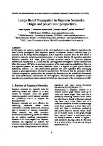
Figure 1: A pairwise Markov random field. Each node represents a random variable, xi . During belief propagation, messages, mij , are sent across edges to convey xi ’s belief in xj ’s current state. A message schedule defines the order these messages are sent. the recipient’s current marginal probability estimate. In graphs with loops (such as Acmi), BP is not guaranteed to arrive at the exact solution, or even converge to any solution. While empirically successful in Acmi, BP is often abandoned in large, complex tasks due to the inability or slowness to converge to a solution. Elidan et al. [9] demonstrated that the manner in which messages are chosen to be processed (or message-passing schedule) can dramatically affect the success of BP. They show that a simple method (e.g., process messages in a roundrobin fashion) is suboptimal, slowing inference in the best case and preventing convergence in the worst case. An efficient scheduler can require fewer message calculations as well as produce better approximations to the true marginal probability distributions. In Figure 1, we see the possible messages that could be sent for a simple graph. The question is: in what order should BP send these messages? Elidan et al. suggested a residual-based method, where each message is prioritized based on how much new information it contains relative to the previous time it was sent. Intuitively, this reduces redundancies and allows BP to identify areas of the graph furthest from convergence. However, we will show this to be ineffective in the fully-connected graph used for Acmi where it produces flat probability distributions that are insufficient for sampling protein structures. We propose, instead, a new method for scheduling messages in belief propagation using domain knowledge. We apply this general framework to the task of performing inference in Acmi, where a prediction of protein disorder [8] can function as a priority function for message passing. We show, across a data set of difficult protein structures, using such a function to prioritize messages in BP improves approximate inference performance in Acmi relative to a naive scheduling protocol. Additionally, informed scheduling results in more complete and accurate protein structures. Section 2 provides background information on interpreting low-resolution electron-density maps, including an overview of Acmi and other methods for automating this task. Section 3 explores belief propagation and discusses protocols for guiding message-passing during the inference phase of Acmi. This section also presents our new method of using domain knowledge to guide BP. Lastly, in Section 4, we compare our
Figure 2: The last step in the protein X-ray crystallography pipeline takes a) the electron-density map (a 3D image) of the protein and finds b) the most likely protein structure that explains the map. Here, the electron density is contoured and the chemical structure of the protein designated with a stick model showing all of the non-hydrogen atoms. new message-passing priority function against our previous work and Elidan et al.’s residual-based protocol across a set of difficult electron-density maps.
2. BACKGROUND 2.1 Automated Density Map Interpretation The last step in the crystallographic process is interpreting the electron-density map, whereby a crystallographer fits a protein molecular model to the density map. This phase is alternatively referred to as tracing the protein. A crystallographer’s task is: given the sequence of the protein and an electron-density map, trace the chain of amino acids through the 3D map. This end goal is the same as in automated ab initio protein-structure prediction, with the difference being that a crystallographer also possesses a fuzzy image of the protein structure. Figure 2 shows a sample density map and the resulting interpretation. Figure 2a) is a contoured electron-density map, similar to what a crystallographer would see at the beginning of interpretation. In b), we see the resulting protein structure with all nonhydrogen atoms in a stick representation. The main chain of atoms is known as the backbone of the protein and the variably sized groups hanging off of the backbone are called side chains. Amino acids (or residues) form the building blocks of proteins, linking end-to-end to form the backbone. Each amino-acid type has a unique side chain molecule, but all connect to the backbone via the Cα atom – the central atom in an amino acid’s structure. Several factors make tracing the protein a difficult and timeconsuming process, mainly by affecting the quality of the electron-density map. The first and most significant factor is the crystallographic resolution of the density map. Crystallographic resolution describes the highest spatial frequency terms used to assemble the electron density map. Resolution is measured in angstroms (˚ A), with higher values indicating poorer-quality maps. Another factor making automation difficult is the phase problem; crystallographer’s can only estimate the phases needed to calculate the electron-density map, reducing the interpretability of the image.
2.2
Other Approaches
Many methods attempt to automate the interpretation of low resolution density maps. The most commonly used method is ARP/wARP [14, 17, 20], an algorithm which iteratively fits structure to a density map, followed by a step of refinement (or improvement) of the map. The algorithm begins by creating a free-atom model – a model containing only unconnected, unlabeled atoms – to fill in the density map of the protein. It then connects some of these atoms, creating a partially-connected backbone. ARP/wARP refines this model, producing a map with improved phase estimates. The process iterates, ending with rotamer search to place side chains and a loop-building phase to connect the chains of atoms [14]. ARP/wARP efficiently finds solutions in maps with 2.7 ˚ A resolution or better, but fails in lower resolution maps when fewer observations are available. Textal [13] uses pattern-recognition techniques in order to interpret maps in the 2.2 to 3.0 ˚ A resolution range. First, Capra [12], a trained neural-network classifier, identifies Cα locations using a set of 19 rotation-invariant features from grid points in the density map. Lookup then identifies side chains by comparing regions of density around each predicted Cα to a database of known side chains and places the best matching side-chain atoms in the trace. Finally, a set of heuristic methods are run to align the structure to the sequence and refine the structure. While the two previous methods use a bottom-up approach, Resolve [23] uses a top-down procedure in which secondarystructure elements are located in the map with the best model being chosen for refinement and extension. Resolve begins by searching the map for a model α-helix and a model β-strand. The next phase of the algorithm extends the best matches using a much larger library of fragments representing helices, strands, and loops. After identifying the highestscoring, non-overlapping segments, Resolve has a backbone trace of the protein. The final step matches each of the Cα atoms in this backbone trace with a likely residue type based on the original sequence and a rotamer library of amino-acid side chains. Resolve has successfully interpreted density maps from 1.1 to 3.2 ˚ A in quality. A recent method, Buccaneer [2], takes a similar approach as Textal by first finding likely Cα locations in the electrondensity map and then extending them into a chain. While Textal utilizes rotation-invariant features to infer Cα positions, Buccaneer utilizes orientation-based features in order to not only infer Cα positions, but the likely orientation of the backbone. Buccaneer currently only performs a backbone trace, and thus does not provide a complete protein model. Results have shown promise on maps ranging up to 3.2 ˚ A in resolution.
2.3
Overview of ACMI
In previous work, DiMaio et al. [4, 5, 6, 7] developed Acmi (Automated Crystallographic Map Interpretation), an alternative approach to density-map interpretation which uses a probabilistic model to trace a protein backbone in poorquality maps (∼3 to 4 ˚ A resolution). Figure 3 provides an overview of Acmi and its three-phase process. Acmi maintains two properties that distinguish it from other methods in the field and allow it to perform inference on diffi-
electron density map, protein sequence ACMI-SH (local match) a priori probability of Cαi’s location ACMI-BP (apply global constraints) marginal probability of Cαi’s location ACMI-PF (sample all-atom structure) protein model Figure 3: The three-phase ACMI pipeline. Given an electron-density map and primary amino-acid sequence, ACMI-SH performs a local-match search independently for each amino acid. The resulting priors are fed to the second phase, ACMI-BP, which applies global constraints to create posterior marginal probabilities of each amino acid’s location. Finally, ACMI-PF uses these marginals to sample physically feasible, all-atom protein structures.
cult maps. First, Acmi simultaneously ties local density information and global constraints to infer possible locations of residues. Second, rather than represent each residue as one or a set of possible locations in the map, Acmi represents each residue’s location as a distribution over the entire electron-density map. This allows the algorithm to overcome poor, early decisions while also allowing weaker evidence to persist and possibly be utilized in later stages. Given an electron-density map and the linear amino-acid sequence of a protein, Acmi builds a pairwise Markov-field model (MRF) [11] to model the location of each amino acid’s Cα atom. A pairwise Markov field, a type of undirected graphical model, defines a probability distribution on a graph. Vertices (or nodes) are associated with random variables, and edges enforce pairwise constraints on those variables. MRF’s are a compact representation of a full-joint probability, allowing for the joint probability function to factorize into smaller functions which can then undergo inference. In Acmi, each vertex corresponds to an amino acid i, and random variables describe the location, u~i , of each Cαi . Figure 4 shows the MRF associated with an example protein. Formally, Acmi’s pairwise Markov-field model G = (V, E) consists of vertices i ∈ V connected by undirected edges (i, j) ∈ E. The full-joint probability of all amino-acid conformations, U, is defined as
P (U|M) =
Y i∈V
ψi (u~i |M) ×
Y (i,j)∈E
ψi,j (u~i , u~j ).
(1)
...
GLU
SER
ALA
THR
ALA
...
Figure 4: A portion of a pairwise Markov field for an example protein sequence. Each node represents a random variable for the configuration (location and orientation) of a residue. Each edge represents a pairwise constraint between the connected random variables. ψi (u~i |M), referred to as the observation potential function, is the function associated with each vertex. It can be thought of as prior probability on the location of an amino acid given the map, M, and ignoring all other amino acids in the protein. Acmi calculates this prior probability in its first phase, Acmi-SH, which performs a shape-matching search of amino acid i at each location in the electron-density map. Briefly, Acmi takes the 5-mer (5-amino-acid sequence) centered at position i in the protein sequence, and searches for exemplar fragments in a non-redundant subset of the Protein Data Bank (PDB) [24]. Each returned fragment is compared to the density map at each grid point, with the maximum correlation coefficient across all rotations being stored. In DiMaio et al. [7], we showed that this six-dimensional search problem can be performed efficiently using spherical-harmonic decompositions [15]. Edge potential functions, denoted ψi,j (u~i , u~j ), represent one of two conformation potentials which define global constraints on the protein structure. Edges between neighboring amino acids in the linear sequence are represented by the adjacency potential function, which encodes the restraint that adjacent residues must maintain an approximate 3.8 ˚ A spacing as well as proper angles. Since amino acids distant in the linear sequence can still neighbor each other in the threedimensional conformation, edges between non-neighboring amino acids contain an occupancy potential. This function reflects the chemical constraint that no two residues can occupy the same space. Acmi, in practice, uses an aggregator function to collect and disseminate occupancy messages efficiently [5]. The model in Equation 1 represents the full-joint probability distribution over all possible configurations (location and orientation) for all residues in the target protein. Calculating this probability exactly, however, is intractable in large graphs with loops. Acmi, instead, employs loopy belief propagation [19], a fast approximate-inference algorithm, to calculate an approximate marginal probability distribution for the location of each amino acid’s Cα atom. This algorithm, Acmi-BP, is the second phase of Acmi and is the crux of this paper. We explore Acmi-BP in Section 3. The original Acmi model in Equation 1 represents just one atom for each residue – the Cα atom. This alone allows for the modeling of a protein’s backbone, but falls short of a complete protein model since it does not model the side-chain atoms. In DiMaio et al. [4], we introduced a
third phase to Acmi, Acmi-PF, which utilizes a sequential sampling algorithm known as particle filtering [1] to produce physically feasible, all-atom, protein structures from the marginal probability distributions resulting from AcmiBP. Our previous results show that the structures produced by the Acmi package are more complete and accurate than all other approaches in the field, across a diverse set of lowresolution electron-density maps [4].
3.
METHODS
Belief propagation is an inference algorithm that calculates marginal probabilities by utilizing a local message-passing scheme to propagate information across a graphical model [19]. A marginal probability represents the posterior probability of a single variable. The terms arises from calculating the full-joint probability and then summing out (or marginalizing) all other variables. In tree-structured graphs, this inference is exact and efficient. In cyclical graphs, such as the model for Acmi, convergence to the exact solution is not guaranteed. In practice, belief propagation in graphs with cycles (loopy belief propagation) tends to produce good approximations, particularly under certain conditions [18]. This section first introduces belief propagation, and the particular notation used for Acmi. Section 3.2 introduces the topic of message scheduling and discusses its impact on the quality of BP’s approximate marginal probabilities. Sections 3.3 and 3.4 discuss informed message-passing protocols for producing improved marginals, including our new domain-knowledge based priority function.
3.1
Belief Propagation Overview
While implementations vary, this section introduces the general outline and notation for belief propagation in AcmiBP. At each iteration, a vertex computes an estimate of its marginal probability distribution as a product over all associated potential functions, marginalizing out other random variables. The vertex then calculates outgoing messages to each of its connected neighbors by combining its marginal probability estimate with the edge potential function shared with that particular neighbor. Acmi-BP, at iteration n for each vertex (i.e., amino acid) i, computes an estimate, pˆn ~i ), of amino acid i’s marginal distribution (or i (u belief ) over locations in the unit cell by combining its local probability and incoming messages:
pˆn ~i ) = ψi (u~i |M) × i (u
Y
mn ~i ) j→i (u
(2)
j∈Γ(i)
where Γ(i) is the set of vertices connected to vertex i. Figure 5 shows a sample message being sent between two amino acids in Acmi, and the resulting update to the receiving node’s belief. Messages from amino acid i to amino acid j are calculated by convoluting the edge potential ψi,j (u~i , u~j ) (i.e., adjacency potential or occupancy potential) with amino acid i’s belief Z mn ~j ) = i→j (u
ψi,j (u~i , u~j ) × EDM
pˆn ~i ) i (u du~i . mn−1 ~i ) j→i (u
(3)
This convolution occurs over the entire distribution, denoted
(a)
LYS31
Algorithm 1: Round-Robin Acmi-BP input : amino-acid sequence Seq of length N , vertex potentials ψi (u~i ) for i = 1 . . . N output: marginal probabilities pˆi (u~i ) for i = 1 . . . N
LEU32
(b)
iter ← 1 while Stop Criteria Not Met do if isOdd(iter) then startRes ← 1; endRes ← N else startRes ← N ; endRes ← 1 end
n mLYS31→LEU32
n pLYS31
n+1 pLEU32
n pLEU32
for i ← startRes to endRes do // Accept messagesQfrom all neighbors pˆi (u~i ) ← ψi (u~i ) × j∈Γ(i) mj→i (u~i )
(c) Figure 5: A sample message being sent in ACMI’s belief propagation algorithm. In a) we show the portion of interest in the protein’s MRF. Here, lysine (node 31) is sending a message to leucine (node 32). In b), we show the current state of beliefs and the calculated message to be sent. Finally, c) shows leucine’s updated belief after receiving the message. The sent message has boosted the confidence in one of the original four peaks. EDM (for Electron-Density Map). The denominator inside the integral removes the influence of the previous message sent across the edge. In essence, a message from vertex i to j is amino acid i stating, “Based on my current belief, I would expect you to be located (with probability) here.”
3.2
Message Scheduling in ACMI-BP
An important design decision for belief propagation is to define a protocol for ordering the passing and receiving of messages. In exact inference, the ordering of messages only affects the rate of convergence, not the final solution. In graph models with loops, however, the message-passing protocol can affect the speed and accuracy of inference [9, 22]. Message-passing protocols fall into two categories: synchronous or asynchronous. Synchronous message passing is where all outgoing messages are calculated at the same time followed by a synchronous reception of messages by all nodes in the graph. Asynchronous message passing, instead, prioritizes messages, sending and updating one at a time. Elidan et al. [9] showed that asynchronous message passing demonstrates faster convergence tendencies and lower error bounds. As shown in Algorithm 1, Acmi-BP utilizes an asynchronous message-passing protocol. In particular, nodes are treated in a simple round-robin fashion where a pass begins at one end of the protein’s primary sequence and works toward the other. At each step along the way, amino acid i first updates its belief based on Equation 2 and then updates its outgoing messages using Equation 3; this sequence is then repeated by amino acid i + 1, and so on. Once all amino acids are processed, the next pass works in the reverse direction. One disadvantage to this protocol is that it does not prioritize
// Calculate messages to all neighbors foreach j ∈ Γ(i) do R ˆi (u ~i ) mi→j (u~j ) = EDM ψi,j (u~i , u~j ) × mpj→i du~i (u ~i ) end end end
nodes based on any metric of evidence or information gain. Even in the best case, this leads to a waste of resources on passing low-information messages along the chain. A more worrying problem arises when the ordering of nodes gives high priority to nodes with poor prior information – that is, false positives in the match search from Acmi-SH. The rest of this section explores alternative scheduling approaches which attempt to identify important messages during the inference process.
3.3
Guiding ACMI-BP using Domain Knowledge
The primary motivation for this work is that well-structured regions of the protein sequence are likely to contain better information in their local match probabilities than disordered regions of the protein. In fact, crystallographers often use such heuristics to decide which portions of the protein molecule to begin placing in the density map [G.N. Phillips and C.A. Bingman, personal communication, 2009]. Portions of the protein structure that are well-structured or ordered have a unique or nearly unique conformation [8]. Disordered regions of structure, conversely, adopt many different conformations under the conditions of the experiment. This often results in smeared density in the protein image since an electron-density map is an average over millions of copies of the protein, each of which takes one of many possible conformations. Thus, the local match search (i.e., Acmi-SH) is unlikely to produce accurate results for disordered amino acids since there is little evidence in the map. To capture this intuition, belief propagation should guide messages based on some domain-knowledge based priority function – that is, some expert determined function of a message’s relevance. If this function is accurate, random variables deemed more influential or a priori more accurate should push belief propagation toward quicker convergence and/or more accurate approximations.
Algorithm 2: Domain-Knowledge Guided Acmi-BP input : amino-acid sequence Seq of length N , vertex potentials ψi (u~i ) for i = 1 . . . N , priority function pord (i) for i = 1 . . . N , decay factor ∆ > 0 output: marginal probabilities pˆi (u~i ) for i = 1 . . . N
lates a residual factor, ri , for each node1 . When a neighbor of i is updated, the residual factor is calculated, capturing the amount of new information available. If that value is larger than the current value for ri , it is updated. ri is defined:
// Priority queue based on function value, paired with node foreach residue i do PQ.push(< pord (i), i >) end while Stop Criteria Not Met do // Pop top value and identify target node, i < val, i >← PQ.pop() // Accept messagesQfrom all neighbors, Γ(i) pˆi (u~i ) ← ψi (u~i ) × j∈Γ(i) mj→i (u~i ) // Calculate messages to all neighbors, Γ(i) foreach j ∈ Γ(i) do R ˆi (u ~i ) mi→j (u~j ) = EDM ψi,j (u~i , u~j ) × mpj→i du~i (u ~i ) end // Add node i back to queue with decayed priority PQ.push(< val − ∆, i >) end
Algorithm 2 shows an overview of our new inference algorithm for guiding Acmi-BP. The main difference from the description in Algorithm 1 is the introduction of a priority measure pord . This probability function is given to AcmiBP by a user. While specifically built for our task, this formulation applies to any instance of belief propagation. The function pord should describe the relative importance of node i in influencing the network. For our task, it measures the probability that amino acid i in a protein’s primary sequence will be well-structured in the final 3D solution. Guided Acmi-BP uses this information to decide, for a given iteration, which residue to next perform inference on. Intuitively, Acmi-BP now focuses the initial iterations on passing information along regions of the sequence likely to produce stable structure. This probability measure is steadily decayed to allow other amino acids to move to the top of the queue. This will allow the (predicted) ordered regions to refine their probabilities, essentially locking in their locations. When less reliable amino acids finally work up the queue, the ordered amino acids should contain more confident messages and thus have a larger influence on the final distributions.
3.4
Related Work
Several methods exist that attempt to improve BP performance by prioritizing nodes based on the amount of new information they expect to receive from their neighbors. Elidan et al. [9] formulated residual belief propagation (RBP), a scheduling function based on the intuition that messages which differ significantly from their previous value are more likely to push BP toward convergence. Conversely, a message whose new value is similar to the value the last time it was sent is contributing relatively little new information to the recipient node and should have low priority. RBP calcu-
old ri = sup kmnew j→i − mj→i k1
(4)
j∈Γ(i)
where Γ(i) is the set of neighbors for node i. At each step of message passing, the node with highest priority is popped off the queue and all of its messages are sent out. This node’s residual value is set to 0, while all neighboring nodes update their beliefs and messages as well as their residual factors if necessary. Further work by Sutton and McCallum [22] approximated these residuals to eliminate unnecessary calculations of new messages that were never sent.
3.5
Experimental Methodology
In Section 4, we compare several variations of belief propagation to determine the effect of a message-passing protocol on Acmi’s ability to produce accurate protein structures. First is the original version of Acmi-BP [6], which uses the round-robin scheduling algorithm in Algorithm 1. In the results in Section 4, this method is designated as BP. We also consider a scheduler based on residual belief propagation [9] from Section 3.4. Algorithm 3 shows the details for applying residual belief propagation to Acmi, where we prioritize nodes according to Equation 4. Acmi-BP scheduled with this function is designated RBP in the results below. Last, we consider a method based on Algorithm 2, utilizing domain knowledge to guide Acmi-BP. In the results below, we denote this heuristic as DOBP (for DisOrder Belief Propagation). Not specified in Algorithm 2 is the source for the input pord (i). This measure would ideally measure the amount of order for amino acid i in the final protein-structure solution. Since we do not know this a priori, we approximate the concept using protein-disorder prediction [8]. Specifically, we use DisEMBL [16], a computational method for disorder prediction using a concept known as “hot loops” – residues without secondary structure (i.e., not a helix or strand) and with high temperature factors. Temperature factors are a term in PDB entries describing the variance of the atom’s location. A higher temperature factor indicates either low confidence by the crystallographer or the existence of multiple conformations. DisEMBL provides reasonable predictions, identifying 60-70% of disordered residues while predicting about 80% of ordered residues [10]. DisEMBL prediction scores are probabilities measuring the likelihood that an amino acid is in a “hot loop” region. In our experiments, the complement of this score is taken to formulate pord (i). For each of the tests in Section 4, all methods use the same Acmi pipeline with the only differences coming in the second phase. First, Acmi-SH is run for each map in the test set 1
While the original formulation maintains a residual for each message, the symmetrical nature of Acmi’s MRF allows us to generalize the method to prioritize nodes.
Algorithm 3: Residual Acmi-BP input : amino-acid sequence Seq of length N , vertex potentials ψi (u~i ) for i = 1 . . . N output: marginal probabilities pˆi (u~i ) for i = 1 . . . N // Initialize priority queue foreach residue i do PQ.push(< 0, i >) end while Stop Criteria Not Met do // Pop top value and identify target node, i < val, i >← PQ.pop() // Accept messagesQfrom all neighbors, Γ(i) pˆi (u~i ) ← ψi (u~i ) × j∈Γ(i) mj→i (u~i ) // Calculate messages and priorities foreach j ∈ Γ(i) do mold ← mi→j (u~j ) R ˆi (u ~i ) du~i mi→j (u~j ) ← EDM ψi,j (u~i , u~j ) × mpj→i (u ~i ) r ← kmi→j − mold k1 if r > PQ.getVal(j) then PQ.remove(j) PQ.push(< r, j >) end end // Add node i back to queue PQ.push(< 0, i >) end
to produce the vertex potentials, according to the protocol in DiMaio et al. [7]. Then, Acmi-BP is run with each of the message-protocols above (i.e., BP, RBP, DOBP) using the same vertex potentials as an input. Each algorithm was run for the equivalent of forty passes across the sequence (i.e., 40 ∗ N nodes were processed). While Acmi-BP could run until convergence, previous results found 40 iterations to be a good stopping point beyond which performance usually did not improve, and sometimes degraded [6]. For results in Section 4.2, Acmi-PF sampled protein structures from the final marginal probability distributions of the respective Acmi-BP methods using the protocol in DiMaio et al. [4]. Each map was run ten times producing a set of ten unique structures, of which the average solution is reported.
4.
RESULTS
To evaluate the different methods for scheduling message passing in belief propagation, we ran each (i.e., BP, RBP, DOBP) in the Acmi framework as described in Section 3.5. We compare the results across the same set of ten difficult protein structures used in DiMaio et al. [4] to show Acmi outperforms all other automated methods in the field. Section 4.1 first details the quality of approximate marginal probability distributions produced using each of the different message-passing protocols. Then, Section 4.2 reports the results of using these marginals in Acmi-PF to produce all-atom protein structures.
4.1
Approximate Marginal Probabilities
As described in Section 2.3, Acmi-BP produces a marginal probability distribution for each amino acid, describing the probability of that amino acid’s location at each point in the electron-density map. Figure 6 shows the log-likelihood of the true solution for each message protocol’s results. This is the probability for the true (i.e., manually traced, PDB deposited) (x,y,z) coordinates for each residue, according to the Acmi-BP produced marginals. The higher this value, the more likely a final trace will place the residue in its correct location. Each point in this figure represents one protein structure, and is an average of log-likelihoods over all residues in that structure. Figure 6a) compares BP to DOBP, with the diagonal line designating equal performance. All points above the line represent maps where DOBP produced higher average-log-likelihoods than BP. In all but two maps, DOBP improved the accuracy of Acmi-BP’s marginal probabilities. In Figure 6b) we see a similar comparison with RBP on the y-axis and BP on x-axis. Here, RBP outperforms BP in 7 of the maps. Figure 6c) shows a mixed picture with RBP and DOBP splitting on the performance across the test set. The overall average-log-likelihood across all maps was -14.5 for BP, -12.0 for DOBP and -12.2 for RBP. In terms of likelihood of the true solution, on average, Acmi-BP benefits from using either informed message-passing protocol.
In our experiments, we use a set of ten experimentally-phased electron-density maps described in DiMaio et al. [4] for validation. This data was provided by the Center for Eukaryotic Structural Genomics (CESG) at UW–Madison. The maps were initially phased using either the Solve [23] or Sharp [3] packages, with non-crystallographic symmetry averaging used to improve the map quality where possible. Based on the electron density quality and quantitative estimate of phase error, expert crystallographers selected these maps as the “most difficult” from a larger data set of twenty maps. These structures have been previously solved and deposited to the PDB, enabling a direct comparison with the correct model2 . However, all ten required a great deal of human effort to build the final atomic model.
One difficulty in comparing average log-likelihood values among different proteins comes from the fact that the size of the probability space for each protein varies. That is, a residue from a protein in a small unit cell has fewer possible outcomes than a protein in a large unit cell. Instead of loglikelihood, we can look at the rank of the true solution since this can be normalized and compared between maps. Figure 7 examines the normalized rank for the true solution of a residue, averaged over all residues in the protein. The rank of the true solution of one residue is the fraction of points in that residue’s marginal probability above the probability of the true solution’s location. Values range from (0, 1] with a rank closest to 0 being the best. The plot in Figure 7 compares BP to DOBP in a), BP to RBP in b), and RBP to DOBP in c). Again, both RBP and DOBP perform better than BP with a relative decrease in rank by 18 and 10 percentage points respectively. That is, BP on average ranks the true residue solution at the 33% mark across all maps while DOBP ranks at the 23% level and RBP at 15%. According to this metric, RBP tends to produce better ranks than DOBP.
2 Test-set solutions were removed from Acmi’s fragment library to blind all methods from the true result.
From these previous results, we can see an improvement in marginal probability accuracy by the RBP and DOBP
-10
-15
(a)
-15
-10
-5
DOBP Log-Likelihood
-5
-20 -20
0
0
RBP Log-Likelihood
DOBP Log-Likelihood
0
-5
-10
-15
-20 -20
0
-15
(b)
BP Log-Likelihood
-5
-10
-5
-10
-15
-20 -20
0
-15
(c)
BP Log-Likelihood
-10
-5
0
RBP Log-Likelihood
Figure 6: Log-likelihoods of the true (i.e., PDB) solution, averaged over all residues in a protein. Each point represents one protein. The shaded region indicates better performance than the original BP protocol for a) using protein-disorder prediction (DOBP) and b) using residual belief propagation (RBP) to guide ACMI-BP. The shaded region of the plot in c) indicates better performance for DOBP relative to RBP.
0.45
0.30
0.15
0
0.45
0.30
0.15
0 0
(a)
0.60
DOBP Solution Rank
0.60
RBP Solution Rank
DOBP Solution Rank
0.60
0.15
0.30
0.45
0.60
0.30
0.15
0 0.15
0
(b)
BP Solution Rank
0.45
0.45
0.30
0.60
0.15
0
(c)
BP Solution Rank
0.30
0.45
0.60
RBP Solution Rank
Figure 7: Normalized rank of the true solution’s probability, averaged over all residues in a protein (see text for definition of rank ). A lower ranking implies the algorithm puts the true locations closer to the most probable location. The shaded area represents better ranks for the true solution relative to BP for a) DOBP and b) RBP. The shaded region in c) shows better ranks for DOBP than RBP.
100
DOBP Completness (%)
DOBP Correctness (%)
100 90 80 70 60
80 70 60 50
50 50
(a)
90
60
70
80
90
BP Correctness (%)
50
100
(b)
60
70
80
90
100
BP Completness (%)
Figure 8: Accuracy of predicted protein structures. Plot a) shows the correctness of predictions – the percent of predicted amino acids within 2 ˚ A of a corresponding residue in the true solution. In b), we plot the completeness of the predictions – the percent of residues from the true solution with a corresponding prediction within 2 ˚ A. The shaded region indicates better performance for DOBP.
message-passing schemes. Biologists, however, are more interested in seeing if this translates into better protein structures at the end of the Acmi pipeline. The final phase of Acmi, Acmi-PF [4], samples all-atom structures from the marginal probabilities produced by Acmi-BP. Unfortunately, this phase of Acmi revealed a shortcoming of RBP. While BP (and DOBP) tend to concentrate probabilities in a few peaks, RBP produced smoother distributions with smaller and more numerous peaks. This is seen in the entropy levels, where the average entropy for an RBP produced marginal was 28.48, over five times higher than the 5.16 and 5.31 averages for DOBP and BP marginals, respectively. The prime culprit is that RBP is susceptible to non-convergent oscillations. That is, a small group of nodes cannot arrive at a stable probability state after a series of messages are passed within this cluster. In this case, the residual stays high in this cluster without resolution, thus choking resources for the other nodes. In fact, for each protein in our set, the median value for the number of times a message was popped off the queue and updated in RBP was either 5 or 6, while the mean was forty. This is problematic for Acmi-PF. To find a good solution, Acmi-PF’s sequential sampling must adequately explore the conformation space of an amino acid. With limited samples, this requires a restricted space of non-negligible locations to search, which is what BP and DOBP provide. RBP, however, contains more locations of non-negligible probability than Acmi-PF can sample in an efficient manner, causing the algorithm to fail. In fact, across all ten proteins, nine failed to produce any portion of the protein structure when using RBP marginals, and the tenth only extended 5% of the total protein. The results in Figure 7 and a histogram of the distributions reflect that RBP excelled at preventing the true solution from having neglible probability (i.e., a rank of 1) and thus looked better on average. RBP, however, did not eliminate enough portions of the density map from consideration for Acmi-PF to succeed. This explains why the rank was much better for RBP, but the log-likelihoods were slightly better for DOBP.
4.2
Protein Structures
After Acmi-BP produces a set of marginal probabilities, Acmi-PF is run to sample physically-feasible protein structures. We compare the accuracy of these protein structures in both completeness and accuracy of the final model for each test-set protein. We compare how Acmi-PF performs with DOBP produced marginals relative to BP produced marginals. As mentioned, RBP did not produce the sharp distributions needed to sample protein structures and thus the results for RBP are not shown below. Figure 8 shows the results of our experiments, with the original Acmi protocol being shown on the x-axis (BP) and the method using domain knowledge for guidance as in Algorithm 2 on the y-axis (DOBP). Each point in the plot refers to one of the test-set proteins. Figure 8a) shows the percent of the predicted protein structure correctly identified. This is akin to the precision of the predicted structures. Precision is a measure of fidelity – that is, of all predictions by algorithm, how many are actually valid? Here, we are describing the percentage of residues predicted that were within 2 ˚ A of their corresponding true solution location. Conversely, Fig-
ure 8b) shows the completeness of the predictions. These are akin to recall – of all possible positive results, how many did the algorithm actually return? For this experiment, we are measuring the percent of residues available in the true (i.e, PDB) solution that were accurately predicted (within 2 ˚ A). Anything above the diagonal indicates DOBP produced better structures. In general, DOBP produced more complete and correct protein structures, particularly in the hardest maps. DOBP did worse on 2 proteins in terms of recall (completeness) and once in terms of precision (correctness). The underperformance in correctness occurs on a structure Acmi was already doing well; in fact, most of the proteins with high correctness did not change one way or the other based on the different marginals. Of the three hardest proteins, however, the correctness was dramatically higher when using DOBP, and in two of these the completeness also improved.
5.
CONCLUSION AND FUTURE WORK
Acmi was previously shown to outperform other methods in the literature in building all-atom protein structures in low quality electron-density maps [4]. The success of Acmi is due to its three-phase probabilistic framework. In this work, we improved the middle phase, Acmi-BP, which combines local match information from the first phase (Acmi-SH) with global constraints to produce a marginal probability of each amino acid’s location in the density map. While Acmi is a successful method, Acmi-BP’s results are only approximations, leaving room to improve the resulting marginal probabilities. The accuracy of these probabilities are crucial for Acmi’s ultimate success as they define the sampling search space for Acmi-PF (the last phase). Results from Elidan et al. [9] indicate that Acmi-BP’s original message-passing protocol was suboptimal and an intelligent protocol could improve BP’s convergence properties. We introduced a general message-passing protocol utilizing domain knowledge to guide belief propagation. We applied this to Acmi-BP by using protein-disorder prediction [8] to favor message passing between amino acids predicted to be well-structured, particularly in the early iterations of BP. Our results indicate that guiding Acmi-BP using this function improves Acmi’s overall performance. Across most maps, the rank and log-likelihood of the true locations of each residue improve. In addition, Acmi is able to build protein structures with improved completeness and correctness from these more accurate approximate marginal probabilities, with the greatest improvement coming in the most difficult test cases. The method proposed by Elidan et al., residual belief propagation [9], fails to produce adequate marginal probabilities for use in Acmi-PF, primarily due to its inability to sufficiently refine the large state space for each amino acid. One avenue of future work is to apply a similar domain knowledge function to Acmi-PF, which utilizes particle filtering – an approximate inference algorithm in which each iteration also requires a choice of what amino acid to next sample in the electron-density map. In addition, we would like to investigate the use of domain-specific heuristics to guide loopy belief propagation when applied to other tasks, particularly other large-state space problems in the computer vision field. Many of these tasks could benefit from our
domain-knowledge message-passing protocol, where rule-ofthumb heuristics can be encoded into a priority function to guide BP.
6.
ACKNOWLEDGMENTS
This research has been supported by NLM grant R01-LM008796 and NLM training grant T15-LM007359. In addition, support for our collaborators at the University of Wisconsin Center for Eukaryotic Structural Genomics (CESG) has been provided by NIH Protein Structure Initiative Grant GM074901. The Acmi system is a collaboration of this paper’s authors and Frank DiMaio, George N. Phillips, Jr., and members of the Phillips Laboratory at the University of Wisconsin– Madison. Acmi and the data set of experimentally-phased density maps is available online at http://pages.cs.wisc.edu/∼dimaio/acmi/get acmi.htm.
7.
REFERENCES
[1] M. Arulampalam, S. Maskell, N. Gordon, and T. Clapp. A tutorial on particle filters. IEEE Transactions of Signal Processing, 50:174–188, 2001. [2] K. Cowtan. The Buccaneer software for automated model building. Acta Crystallographica, D62:1002–1011, 2006. [3] E. de La Fortelle and G. Bricogne. Maximum-likelihood heavy-atom parameter refinement for the multiple isomorphous replacement and multiwavelength anomalous diffraction methods. Methods in Enzymology, 276:472–494, 1997. [4] F. DiMaio, D. Kondrashov, E. Bitto, A. Soni, C. Bingman, G. Phillips, and J. Shavlik. Creating protein models from electron-density maps using particle-filtering methods. Bioinformatics, 23:2851–2858, 2007. [5] F. DiMaio and J. Shavlik. Belief propagation in large, highly connected graphs for 3D part-based object recognition. In Proceedings of the Sixth IEEE International Conference on Data Mining, pages 845–850, Hong Kong, 2006. [6] F. DiMaio, J. Shavlik, and G. N. Phillips. A probabilistic approach to protein backbone tracing in electron-density maps. Bioinformatics, 22(14):e81–89, 2006. [7] F. DiMaio, A. Soni, G. N. Phillips, and J. Shavlik. Spherical-harmonic decomposition for molecular recognition in electron-density maps. International Journal of Data Mining and Bioinformatics, 3(2):205–227, 2009. [8] A. K. Dunker, E. Garner, S. Guilliot, P. Romero, K. Albrecht, J. Hart, Z. Obradovic, C. Kissinger, and J. E. Villafranca. Protein disorder and the evolution of molecular recognition: Theory, predictions and observations. Pacific Symposium on Biocomputing, pages 473–484, 1998. [9] G. Elidan, I. McGraw, and D. Koller. Residual belief propagation: Informed scheduling for asynchronous message passing. In Proceedings of the Twenty-Second Conference on Uncertainty in Artificial Intelligence, pages 165–173, 2006. [10] F. Ferron, S. Longhi, B. Canard, and D. Karlin. A practical overview of protein disorder prediction methods. Proteins: Structure, Function, and
Bioinformatics, 65(1):1–14, 2006. [11] S. Geman and D. Geman. Stochastic relaxation, Gibbs distributions, and the Bayesian restoration of images. IEEE Transactions on Pattern Analysis and Machine Intelligence, 6:721–741, 1984. [12] T. Ioerger and J. Sacchettini. Automatic modeling of protein backbones in electron density maps via prediction of C-alpha coordinates. Acta Crystallographica, D58:2043–2054, 2002. [13] T. Ioerger and J. Sacchettini. The Textal system: Artificial intelligence techniques for automated protein model building. Methods in Enzymology, 374:244–270, 2003. [14] K. Joosten, S. Cohen, P. Emsley, W. Mooij, V. Lamzin, and A. Perrakis. A knowledge-driven approach for crystallographic protein model completion. Acta Crystallographica, D64:416–424, 2008. [15] A. Kirillov. Representation Theory and Noncommutative Harmonic Analysis, volume 22 of Encyclopedia of Mathematical Sciences. Springer, 1994. [16] R. Linding, L. J. Jensen, F. Diella, P. Bork, T. J. Gibson, and R. B. Russell. Protein disorder prediction: Implications for structural proteomics. Structure, 11(11):1453–1459, 2003. [17] R. Morris, A. Perrakis, and V. Lamzin. ARP/wARP and automatic interpretation of protein electron density maps. Methods in Enzymology, 374:229–244, 2003. [18] K. Murphy, Y. Weiss, and M. Jordan. Loopy belief propagation for approximate inference: An empirical study. In Proceedings of the Fifteenth Conference on Uncertainty in Artificial Intelligence, pages 467–475, 1999. [19] J. Pearl. Probabilistic Reasoning in Intelligent Systems: Networks of Plausible Inference. Morgan Kaufman Publishers, San Mateo, CA, 1988. [20] A. Perrakis, R. Morris, and V. Lamzin. Automated protein model building combined with iterative structure refinement. Nature Structural and Molecular Biology, 6(5):458–463, 1999. [21] Protein Data Bank (PDB). PDB current holdings breakdown. http://www.rcsb.org/pdb/statistics/holdings.do, August 2009. [22] C. Sutton and A. McCallum. Improved dynamic schedules for belief propagation. In Proceedings of the Twenty-Third Conference on Uncertainty in Artificial Intellignece, 2007. [23] T. C. Terwilliger. Automated main-chain model building by template matching and iterative fragment extension. Acta Crystallographica, D59:38–44, 2003. [24] G. Wang and R. J. Dunbrack. Pisces: A protein sequence culling server. Bioinformatics, 19:1589–1591, 2003.