some problems significantly faster than using set bounds propagation because of the ... denoted D1 = D2, if D1(v) = D2(v) for all variables v. We also use range ...
Set Domain Propagation Using ROBDDs Vitaly Lagoon and Peter J. Stuckey Department of Computer Science and Software Engineering The University of Melbourne, Vic. 3010, Australia {lagoon,pjs}@cs.mu.oz.au
Abstract. Propagation based solvers typically represent variables by a current domain of possible values that may be part of a solution. Finite set variables have been considered impractical to represent as a domain of possible values since, for example, a set variable ranging over subsets of {1, . . . , N } has 2N possible values. Hence finite set variables are presently represented by a lower bound set and upper bound set, illustrating all values definitely in (and by negation) all values definitely out. Propagators for finite set variables implement set bounds propagation where these sets are further constrained. In this paper we show that it is possible to represent the domains of finite set variables using reduced ordered binary decision diagrams (ROBDDs) and furthermore we can build efficient domain propagators for set constraints using ROBDDs. We show that set domain propagation is not only feasible, but can solve some problems significantly faster than using set bounds propagation because of the stronger propagation.
1
Introduction
Many constraint satisfaction problems are naturally expressed using set variables and set constraints, where the set variables range over subsets of a given a finite set of integers. One widely-adopted approach to solving CSPs combines backtracking tree search with constraint propagation. Constraint propagation, based on local consistency algorithms, removes infeasible values from the domains of variables to reduce the search space. One of the most successful consistency techniques is domain consistency [14] which ensures that for each constraint c, every value in the domain of each variable can be extended to an assignment satisfying c. For simplicity, we refer to constraint propagation based on domain consistency as domain propagation. Propagators are functions to perform constraint propagation. Unfortunately domain propagation where the variables range over sets is usually considered infeasible. For example, if a variable must take as a value a subset of {1, . . . , N } there are 2N possible values. Simply representing the domain of possible values seems to be impractical. For this reason constraint propagation over set variables is always, as far as we are aware, restricted to use set bounds propagation [6, 11].
In set bounds propagation, a set variable v has its domain represented by two sets L the least possible set (that is all the values that must be in the set v) and U the greatest possible set (that is the complement of all values that cannot be in set v). Set bounds propagators update the least and greatest possible sets of variables v according to the constraints in which they are involved. Interestingly set bounds propagation as defined in [6] is equivalent to modelling the problem using Boolean constraints and applying domain propagation to these constraints. That is the set variable v is represented by N Boolean variables v1 , . . . , vN which represent the propositions vi ⇔ i ∈ v. Refined versions of set bounds propagation, that add a representation of the cardinality of a variable to its domain, such as [1, 10], give stronger propagation. In this paper we investigate this Boolean modelling approach further. We show it is possible to represent the domains of finite set variables using reduced ordered binary decision diagrams (ROBDDs). We shall show that domains can be represented by very small ROBDDs, even if they represent a large number of possible sets. Furthermore we represent set constraints using ROBDDs, and use this to build efficient domain propagators for set constraints. ROBDD representations of simple set constraints are surprisingly compact. In summary the contributions of this paper are: – We show how to efficiently representing domains of (finite) set variables using ROBDDs. – We show that we can build efficient constraint propagators for primitive set constraints using ROBDDs – We illustrate the wealth of modelling possibilities that arise using ROBDDs to build propagators. – We give experiments illustrating that set domain propagation is advantageous for (finite) set constraint problems.
2
Preliminaries
In this paper we consider finite set constraint solving (over sets of integers) with constraint propagation and tree search. Let V denote the set of all set variables. Each variable is associated with a finite set of possible values (which are themselves sets), defined by the domain of the CSP. A domain D is a complete mapping from a fixed (countable) set of variables V to finite sets of finite sets of integers. The intersection of two domains D1 and D2 , denoted D1 u D2 , is defined by the domain D3 (v) = D1 (v) ∩ D2 (v) for all v. A domain D1 is stronger than a domain D2 , written D1 v D2 , if D1 (v) ⊆ D2 (v) for all variables v. A domain D1 is equal to a domain D2 , denoted D1 = D2 , if D1 (v) = D2 (v) for all variables v. We also use range notation whenever possible: [L .. U ] denotes the set of sets of integers {d | L ⊆ d ⊆ U } when L and U are sets of integers. We shall be interested in the notion of an initial domain, which we denote Dinit . The initial domain gives the initial values possible for each variable. In effect an initial domain allows us to restrict attention to domains D such that
D v Dinit . For our purposes we shall restrict attention to initial domains Dinit where Dinit (x) = [∅ .. {1, . . . , N }] for all variables x. A valuation θ is a mapping of variables to sets of integer values, written {x1 7→ d1 , . . . , xn 7→ dn }. We extend the valuation θ to map expressions or constraints involving the variables in the natural way. Let vars be the function that returns the set of variables appearing in an expression, constraint or valuation. In an abuse of notation, we define a valuation θ to be an element of a domain D, written θ ∈ D, if θ(vi ) ∈ D(vi ) for all vi ∈ vars(θ). Constraints A constraint places restriction on the allowable values for a set of variables and is usually written in well understood mathematical syntax. For our purposes we shall restrict ourselves to the following primitive set constraints: (element) k ∈ v, (not element) k 6∈ v, (equality) v = w, (constant) v = d, (subset) v ⊆ w, (union) u = v ∪ w, (intersection) u = v ∩ w, (subtraction) u = v − w, (complement) v = w, (disequality) v 6= w, (cardinality equals) |v| = k, (cardinality lower) |v| ≥ k, and (cardinality upper) |v| ≤ k, where u, v, w are set variables, d is a constant finite set and k is a constant integer. A set constraint is a (possibly existentially quantified) conjunction of primitive set constraints. Later we shall introduce more complex forms of set constraint. We define solns(c) = {θ | vars(θ) = vars(c)∧ |=θ c}, that is the set of θ that make the constraint c hold true. We call solns(c) the solutions of c. Propagators and Propagation Solvers In the context of propagation-based constraint solving, a constraint specifies a propagator, which gives the basic unit of propagation. A propagator f is a monotonically decreasing function from domains to domains, i.e. D1 v D2 implies that f (D1 ) v f (D2 ), and f (D) v D. A propagator f is correct for constraint c iff for all domains D {θ | θ ∈ D} ∩ solns(c) = {θ | θ ∈ f (D)} ∩ solns(c) This is a weak restriction since for example, the identity propagator is correct for all constraints c. Example 1. For S the constraint c ≡ v ⊆ w the function f (D)(v) = {d1 ∈ D(v) | d1 ⊆ D(w)}, f (D)(w) = D(w), is a correct propagator for c. Let D1 (v) = {{1}, {1, 3, 5}, {6}, {3, 4}} and D1 (w) = {{1}, {3, 4, 5}, {2}}, then f (D1 ) = D2 where D2 (v) = {{1}, {1, 3, 5}, {3, 4}} and D2 (w) = D1 (w). A propagation solver for a set of propagators F and current domain D, solv (F, D), repeatedly applies all the propagators in F starting from domain D until there is no further change in resulting domain. solv (F, D) is the largest domain D 0 v D which is a fixpoint (i.e. f (D 0 ) = D0 ) for all f ∈ F . In other words, solv (F, D) returns a new domain defined by iter (F, D) =
l f ∈F
f (D)
and
solv (F, D) = gfp(λd.iter (F, d))(D)
where gfp denotes the greatest fixpoint w.r.t v lifted to functions. Domain Consistency A domain D is domain consistent for a constraint c if D is the least domain containing all solutions θ ∈ D of c, i.e, there does not exist D0 @ D such that θ ∈ D ∧ θ ∈ solns(c) → θ ∈ D 0 . A set of propagators F maintains domain consistency for a constraint c, if solv (F, D) is always domain consistent for c. Define the domain propagator for a constraint c as dom(c)(D)(v) = {θ(v) | θ ∈ D ∧ θ ∈ solns(c)} where v ∈ vars(c) dom(c)(D)(v) = D(v) otherwise Example 2. For the constraint c ≡ v ⊆ w and let D3 = dom(c)(D1 ) where D1 (v) = {{1}, {1, 3, 5}, {6}, {3, 4}} and D1 (w) = {{1}, {3, 4, 5}, {2}}, then D3 (v) = {{1}, {3, 4}} and D3 (w) = {{1}, {3, 4, 5}}. Now D3 is domain consistent with respect to c. Set Bounds Consistency Domain consistency has been considered prohibitive to compute for constraints involving set variables. For that reason, set bounds propagation [6, 10] is typically used where a domain maps a set variable to a lower bound set of integers and an upper bound set of integers. We shall enforce this by treating the domain D(x) of a set variable x as if it were the range [∩D(x) .. ∪ D(x)]. In practice if only set bounds propagators are used, all domains will be of this form in any case. Define ran(D) as the domain D0 where D 0 (x) = [∩D(x) .. ∪ D(x)]. The set bounds propagator returns the smallest set range which includes the result returned by the domain propagator. Define the set bounds propagator for a constraint c as sb(c)(D)(v) =
D(v) ∩ v ∈ vars(c) [∩dom(c)(ran(D))(v) .. ∪ dom(c)(ran(D))(v)]
sb(c)(D)(v) = D(v) otherwise Example 3. Given constraint c ≡ v ⊆ w and D4 = sb(c)(D1 ), where D1 is defined in Example 2. Then ran(D1 )(v) = [∅ .. {1, 3, 4, 5, 6}], ran(D1 )(w) = [∅ .. {1, 2, 3, 4, 5}], D4 (v) = {{1}, {1, 3, 5}, {3, 4}} and D4 (w) = {{1}, {3, 4, 5}, {2}}. Boolean Formulae and Binary Decision Diagrams We make use of the following Boolean operations: ∧ (conjunction), ∨ (disjunction), ¬ (negation), → (implication), ↔ (bi-implication) and ∃ (existential quantification). We denote by ∃ V F ¯V F we mean ∃V 0 F the formula ∃x1 · · · ∃xn F where V = {x1 , . . . , xn }, , and by ∃ 0 where V = vars(F ) − V . The Reduced Ordered Binary Decision Diagram (ROBDD) [3] is a canonical representation of Boolean function. An ROBDD is a directed acyclic graph. There are two terminal nodes are labeled with the Boolean constants 0 (false) and 1 (true). Each non-terminal node is labelled by a variable and has two branches,
a 1-branch and a 0-branch, corresponding respectively to the two possible values of the variable. Thus, the value of a Boolean function for a given assignment of variables can be computed as a terminal reached from the root by following the corresponding 1- or 0-branches. An ROBDD obeys the following restrictions: – Variables are totally ordered by some ordering ≺ and each child node (with label w) of a node labelled v is such that v ≺ w. – There are no duplicate subgraphs (nodes with the same variable label and 1- and 0-branches). – There are no redundant tests (each non-terminal node has different 1- and 0-branches). Example 4. The ROBDD for the formula (v1 → w1 ) ∧ (v2 → w2 ) with the ordering of variables v1 ≺ v2 ≺ w1 ≺ w2 is shown in Figure 2(a). The ROBDD is read as follows. Each non-leaf node has a decision variable. If the variable is false (0) we take the left 0-branch (dashed), if the variable is true (1) we take the right 1-branch (solid). One can verify that for example a valuation that make the formula true, e.g. {v1 7→ 1, v2 7→ 0, w1 7→ 1, w2 7→ 1}, give a path to the node 1, while valuations that make the formula false, e.g. {v1 7→ 0, v2 7→ 1, w1 7→ 1, w2 7→ 0}, give a path to the node 0. The ROBDD-based representations of Boolean functions are canonical meaning that for a fixed order of variables two Boolean functions are equivalent if and only if their respective ROBDDs are identical. There are efficient algorithms for many Boolean operations applied to ROBDDs. Let |r| be the number of internal nodes in ROBDD r then the complexity of the basic operations for constructing new ROBDDs is O(|r1 ||r2 |) for r1 ∧ r2 , r1 ∨ r2 and r1 ↔ r2 , O(|r|) for ¬r, and O(|r|2 ) for ∃x.r. Note however that we can test whether two ROBDDs are identical, whether r1 ↔ r2 is equivalent to true (1), in O(1). Although in theory the number of nodes in an ROBDDs can be exponential in the number of variables in the represented Boolean function, in practice ROBDDs are often very compact and computationally efficient. This is due to the fact that ROBDDs exploit to a very high-degree the symmetry of models of a Boolean formula.
3 3.1
Basic Set Domain Propagation Modelling Set Domains using ROBDDs
The key step in building set domain propagation using ROBDDs is to realise that we can represent a finite set domain using an ROBDD. Let x be a set variable taking a value A subset of {1, . . . , N }, then we can represent A using a valuation θA of the vector of Boolean variables V (x) = hx1 , . . . , xN i, where θA = {xi 7→ 1 | i ∈ A} ∪ {xi 7→ 0 | i 6∈ A}. We can represent an arbitrary set of subsets S of {1, . . . , N } by a Boolean formula φ which has
(/x).*+-,EE 1
£ ¯ Â
¸ )
(/x).*+-,Ey| E 3
£
(/).*+-,
EE " x y 2
2§ ¼N < Ã Z.0
(a)
(/).*+-,
(/).*+-,
EE " x z 5 AAA AÃ |qz
1
(/).*+-,
s z 1 DDD D! }z s2 D s z DD z 2 DDD D D! }z ! }z s3 D s3 D s z DD z3 z DD D D }z ! }z ! }z s4 D s4 s4 D D D z z DD · DD z z } } ! ! ¹ s5 C s CC {5 ² À C! }{ ' ¹ 1 7 1 M X V _ ]a /0 0 spo
(/).*+-,
(/).*+-,
(/).*+-,
(/).*+-,
(/).*+-,
(/).*+-,
(/).*+-,
(/).*+-,
(/).*+-,
(b)
Fig. 1. ROBDDs for (a) [{1, 3, 5} .. {1, 3, . . . N }] and (b) (s ⊆ {1, 2, 3, 4, 5} , |s| = 2).
exactly the solutions {θA | A ∈ S}. We will order the variables x1 ≺ x2 · · · ≺ xN . For example the set of sets S = {{1, 2}, {}, {2, 3}} where N = 3 is represented by the formula (x1 ∧ x2 ∧ ¬x3 ) ∨ (¬x2 ∧ ¬x2 ∧ ¬x3 ) ∨ (¬x1 ∧ x2 ∧ x3 ). An ROBDD allows us to represent (some) subsets of 2{1,...,N } efficiently. The initial domain for x, Dinit (x) = [∅ .. {1, . . . , N }], is represented by the O(1) sized ROBDD 1, independent of N . If D(x) = [{1, 3, 5} .. {1, 3, . . . , N }], we can represent these 2N −4 sets by the ROBDD shown in Figure 1(a), again independent of N . Indeed any domain D0 (x) of the form [L .. U ] can be represented in O(|L| + N − |U |). Even some sets of subsets that may appear difficult to represent are also representable efficiently. Consider representing all the subsets of {1, 2, 3, 4, 5} of cardinality 2. Then the ROBDD representing this domain is shown in Figure 1(b). 3.2
Modelling Primitive Set Constraints using ROBDDs
We will convert each primitive set constraint c to an ROBDD B(c) on the Boolean variable representations V (x) of its set variables x. We must be careful in ordering the variables in each ROBDD in order to build small representations of the formula. Example 5. Consider the two representations of the ROBDD for the constraint representing v ⊆ w where Dinit (v) = Dinit (w) = [∅ .. {1, 2}] shown in Figure 2. The first representation with the ordering v1 ≺ v2 ≺ w1 ≺ w2 is much larger than the second with ordering v1 ≺ w1 ≺ v2 ≺ w2 . In fact if we generalize for initial domains of size N the ordering v1 ≺ · · · ≺ vN ≺ w1 ≺ · · · ≺ wN leads to an exponential representation, while the order v1 ≺ w1 ≺ v2 ≺ w2 ≺ · · · ≺ vN ≺ wN is linear.
(/).*+-,
v y 1 EEEE y E" |y v2 RR RRR yv2 EEEE R|yRyR ° E" R w1 E RRRRR w1 F » " } EEE y yRRRRFRFFF R) # EEy , ÂÄ y EEE h h h w2 : ? J AÃ |y yh h hEE" V - sh 0 1o
(/).*+-,
(/).*+-,
(/).*+-,
(/).*+-,
(/).*+-,
(a) Order: v1 ≺ v2 ≺ w1 ≺ w2
(/v).*+-,$ EEE 1
+
(/).*+-,
EE " w1 E EEE ¢ ®E [ a E1 " v 2E E Â · EEE" ¾ w2 3 2 ¡ = Ä Ã o _ _ mS Z . v 0
(/).*+-,
0123 7654 1
(b) Order: v1 ≺ w1 ≺ v2 ≺ w2
Fig. 2. Two ROBDDs for v ⊆ w
By ordering the Boolean variables pointwise we can guarantee linear representations B(c) for each primitive constraint c except those for cardinality. The table of expressions and sizes is shown in Figure 3. The cardinality primitive constraints use a subsidiary Boolean formula defined by the function card (v, l, u, n) which is the cardinality of v restricted to the elements from n + 1, . . . , N is between l and u. It is defined recursively as follows: 1 if l ≤ 0 ∧ N − n ≤ u 0 if N − n < l ∨ u < 0 card (v, l, u, n) = (¬v ∧ card (v, l, u, n + 1)) ∨ n+1 otherwise (vn+1 ∧ card (v, l − 1, u − 1, n + 1)
This definition also shows why the representation is quadratic since the right hand sides directly represent ROBDD nodes. For any formula card (v, l, u, n) it involves at most a quadratic number of subformulæ. 3.3
Basic Set-Domain Solver
We build a domain propagator dom(c) for constraint c using ROBDDs as follows. Let vars(c) = {v1 , . . . , vn } then we define ¯V (v ) .B(c) ∧ Vn D(vj ) dom(c)(D)(vi ) = ∃ i j=1
This formula directly defines the domain consistency operator. Because each of B(c) and D(vj ) is an ROBDD this is directly implementable using ROBDD operations. Example 6. Assume N = 2 and suppose D(v) = {{1}, {1, 2}}, and D(w) = [∅ .. {1, 2}], represented by the ROBDDs v1 and 1. We conjoin these with the ROBDD for v ⊆ w shown in Figure 2(c) (the result is a similar ROBDD with left child of the root 0). We project this ROBDD onto the Boolean variables w1 , w2
c Boolean expression B(c) k∈v vk ¬v k 6∈ v Vk v=w (vi ↔ wi ) V1≤i≤N V v ∧ v=d i 1≤i≤N,i6∈d ¬vi Vi∈d (v → wi ) v⊆w i V1≤i≤N u=v∪w (u ↔ (vi ∨ wi )) i V1≤i≤N u=v∩w (u ↔ (vi ∧ wi )) i V1≤i≤N u=v−w (ui ↔ (vi ∧ ¬wi )) 1≤i≤N V v=w ¬(vi ↔ wi ) W1≤i≤N v 6= w 1≤i≤N ¬(vi ↔ wi ) |v| = k card (v, k, k, 0)) |v| ≥ k card (v, k, N, 0) |v| ≤ k card (v, 0, k, 0)
size of ROBDD O(1) O(1) O(N ) O(N ) O(N ) O(N ) O(N ) O(N ) O(N ) O(N ) O(k(N − k)) O(k(N − k)) O(k(N − k))
Fig. 3. Boolean representation of set constraints and size of ROBDD.
of w obtaining the formula w1 . The new domain of W becomes w1 representing sets {{1}, {1, 2}}. The basic propagation mechanism improves slightly on the mathematical definition by (a) only revisiting propagators when the domain of one of their variables changes (b) ensuring that the last propagator is not re-added by its own changes since it is idempotent. We can also execute unary constraint propagators just once. The code for solv is shown below where for simplicity the first argument is a set of constraints, rather than their domain propagators. solv(C, D) Q := C while (∃c ∈ Q) D0 := dom(c)(D) V := {v ∈ V | D(v) 6= D 0 (v)} Q := (Q ∪ {c0 ∈ C | vars(c0 ) ∩ V 6= ∅}) − {c} D := D 0 return D Note that detecting the set V of variables changed by the dom(c) is cheap because the equivalence check D(v) = D 0 (v) for ROBDDs is constant time (the two pointers must be identical).
4 4.1
Towards a More Efficient Set Domain Solver Removing Intermediate Variables
For many real problems the actual problem constraints will not be primitive set constraints, but rather more complicated set constraints that can be split
into primitive set constraints. This means that we introduce new variables and multiple propagators for a single problem constraint. Example 7. Consider the following constraint |v ∩ w| ≤ 1 which is found in many problems, requiring that v and w have at most one element in common. This can be represented as primitive set constraints by introducing an intermediate variable u as ∃u.u = v ∩ w ∧ |u| ≤ 1. For set bounds propagation this breaking down of the constraint is implicitly performed. Now the splitting into primitive constraints does not affect the propagation strength of the resulting set of propagators. But it does add a new variable, and complicate the propagation process by making more constraints. Using an ROBDD representation of the more complex constraint we can avoid splitting the constraint. Instead we construct a Boolean representation directly using ROBDD operations. Essentially we can take the ROBDDs for the individual primitive constraints and project away the intermediate variable. Example 8. We can build a propagator dom(c) directly for the constraint c ≡ |v ∩ w| ≤ 1, by constructing the ROBDD ∃V (u) .B(u = v ∩ w) ∧ B(|u| ≤ 1). The resulting ROBDD has size O(N ). This contrasts with set bounds propagation where we must carefully construct a new propagator for each kind of primitive constraint we wish to support. Typically only the given primitive constraints are provided and intermediate variables are silently introduced. This approach is used for instance in set constraint solvers provided by ECLi PSe [5]. 4.2
Building Global Constraints
Just as we can create more complex ROBDDs for constraints that are typically broken up into primitive sets constraints, we can also build domain propagators for complex conjunctions of constraints using ROBDD operations, so called global constraints. Example 9. Consider the following constraint partition(v1 , . . . , vn ) which requires that the sets v1 , . . . , vn form a partition of {1, . . . , N }. The meaning in terms of primitive set constraints is Vn V n ij .uij = vi ∩ vj ∧ uij = ∅) ∧ j=i+1 (∃uV i=1 n ∃w1 . . . wn+1 .wn+1 = ∅ ∧ i=1 (wi = vi ∪ wi+1 ) ∧ w1 = {1, . . . , N }
Now dom(partition(v1 , . . . , vn )) is much stronger in propagation than the set of propagators for the primitive constraints in its definition. For example consider partition(v1 , . . . , v3 ) and domain D where D(v1 ) = D(v2 ) = {{1}, {2}} and D(v3 ) = {{2}, {3}} and N = 3. While the individual propagators will not modify the domain, the global propagator will revise the domain of v3 to {{3}}. We can build a single ROBDD (of size O(nN )) representing this formula, and hence we have built a domain constructor for the entire constraint.
Clearly as we build larger and larger global constraint propagators we will build larger and larger ROBDD representations. There is a tradeoff in terms of strength of propagation versus time to propagate using this ROBDD. Example 10. Consider the constraint atmost([v1 , . . . , vn ], k) introduced in [12], which requires that each of the n sets of cardinality k should intersect pairwise in at most one element. The meaning in terms of primitive set constraints is Vn Vn Vn j=i+1 (∃uij .uij = vi ∩ vj ∧ |uij | ≤ 1) i=1 |vi | = k ∧ i=1 While we can create an ROBDD that represents the entire global constraint the resulting ROBDD is exponential in size. Hence it is not practical to use as a global propagator. 4.3
Breaking Symmetries with Order Constraints
In many problems involving set constraints there will be large numbers of symmetries which can substantially increase the size of the search space. One approach to removing symmetries is to add order constraints v < w among sets. v < w means that the list of Booleans V (v) is lexicographically smaller than the list of Booleans V (w). These order constraints can be straightforwardly represented using ROBDDs of size O(N ). We represent v < w by the formula ltset(v, w, 1) where ½ 0 n>N ltset(v, w, n) = (¬vn ∧ wn ) ∨ ((vn ↔ wn ) ∧ ltset(v, w, n + 1)) otherwise
5
Experiments
We have implemented a set-domain solver based on the method proposed in this paper. Our implementation written in Mercury [13] integrates a fairly na¨ıve propagation-based mechanism with an ROBDD library. We have chosen the CUDD package [4] as a platform for ROBDD manipulations. We conducted a series of experiments using our solver and compared the experimental results with the data collected by running the ECLi PSe [5] ic sets set bounds propagation solver on the same problems. All experiments were conducted on a machine with Pentium-M 1.5 GHz processor running Linux v2.4. 5.1
Ternary Steiner Systems
A ternary Steiner system of order N is a set of N (N − 1)/6 triplets of distinct elements taking their values between 1 and N , such that all the pairs included in two different triplets are different. A Steiner triple system of order N exists if and only if n ≡ 1, 3 mod 6, as shown by Kirkman [7]. A ternary Steiner system of order N is naturally modelled using set variables s1 . . . sm , where m = N (N − 1)/6 and constrained by: Vm Vm−1 Vm j=i+1 (|si ∩ sj | ≤ 1 ∧ (si < sj )) i=1 (|si | = 3) ∧ i=1
Table 1. ROBDD set domain solver for finding Steiner systems. The simple model with separate constraints and intermediate variables. “element in set” labeling Problem
Model size ×103
steiner(7) steiner(9) steiner(13) steiner(15)
3 11 47 140
“element not in set” labeling
sequential first-fail sequential first-fail time fails size time fails size time fails size time fails size sec.
×103
0.1 1 18 4.6 365 324 — — — — — —
sec.
×103
sec.
×103
sec.
×103
0.0 1 18 0.0 0 16 0.0 0 16 4.7 370 325 1.3 100 180 1.4 100 180 — — — — — — — — — — — — 23.9 0 1,058 24.1 0 1,058
where we have added ordering constraints si < sj to remove symmetries. We conducted a series of experiments finding the first solution for Steiner systems of orders 7,9,13 and 15. We use four labeling strategies given by crosscombinations of two ways of choosing a variable for labeling and two modes of assigning values. The choice of variable is either sequential or “first-fail” i.e., a variable with a smallest domain is chosen at each labeling step. Once a variable is chosen we explore the two possibilities for each possible element of set from least to greatest. Each element is either a member of the set represented by the variable, or it is not. The alternative (element in set) or (element not in set) we try first induces the two modes of value assignment. This order is significant in practice, as we show in our experiments. Table 1 summarizes the experimental data produced by our BDD-based solver for the model where each primitive set constraint is represented separately and intermediate variables are introduced (see Example 7). For each problem we provide the size of the corresponding model. The sizes listed in this and the following tables are measured in the number of (thousands of) ROBDD nodes. For each run we count the run-time, the number of fails i.e., the number of times the solver backtracks from its choice of value, and the maximum number of live ROBDD nodes reached during the run. The “—” entries correspond to runs which could not complete in ten minutes. A better ROBDD model of the constraints for the Steiner problem merges the constraints on each pair si and sj , constructing a single ROBDD for each ψij = (|si ∩ sj | ≤ 1) ∧ (si < sj ), and avoiding the intermediate variable. The results using this model are shown in Table 2. While the resulting model can be larger, the search space is reduced since dom(ψij ) propagates more strongly than the set {dom(|si ∩ sj | ≤ 1), dom(si < sj )}, and the time and peak size usage is substantially decreased. Hence it is clearly beneficial to eliminate intermediate variables and merge constraints. We compared the set domain propagation solver against the ECLi PSe set bounds propagation solver ic sets using the same model and search strategies. We had to implement a version of v < w for sets using reified constraints. Table 3 shows the corresponding results to Table 2.
Table 2. ROBDD set domain solver for finding Steiner systems. The improved model with merged constraints and no intermediate variables. “element in set” labeling Problem
Model size ×103
steiner(7) steiner(9) steiner(13) steiner(15)
“element not in set” labeling
sequential first-fail sequential first-fail time fails size time fails size time fails size time fails size sec.
3 11 76 92
0.0 0.0 — 2.8
×103
sec.
×103
sec.
×103
sec.
×103
0 4 0.0 0 4 0.0 0 4 0.0 0 4 2 17 0.1 798 23 0.1 9 20 0.1 9 20 — — 336.3 21,264 398 160.5 24,723 295 80.2 6,195 288 0 172 — — — 2.2 0 160 2.4 0 160
Table 3. ECLi PSe set bounds solver for finding Steiner systems. “element in set”
“element not in set”
Problem
sequential first-fail sequential first-fail time fails time fails time fails time fails steiner(7) 0.0 9 0.0 9 0.0 10 0.0 10 steiner(9) 1.0 542 1.2 542 4.9 1,394 4.8 1,394 steiner(13) — — — — — — — — steiner(15) 2.4 6 33.9 7,139 2.8 65 3.4 65
Clearly the set domain solver involves far less search than the set bounds solver. It is also able to find solutions to the hardest example steiner(13). The set domain solver is faster than set bounds solving except for steiner(15) with sequential labeling, and when with first-fail labeling it gets stuck in a very unproductive part of the search space. One should note that with first-fail labeling the search spaces explored are quite different, since the variable ordering changes. In order to better gauge the relationship between the two approaches without being biased by search strategy we ran experiments to find all distinct Steiner systems of orders 7 and 9 modulo the lexicographic ordering. Table 4 summarizes the results of the experiments. We list the best results for the both solvers. The results are in both cases are obtained using the “first-fail” and “element not in set” labeling strategy. The run of the ECLi PSe solver for N = 9 was aborted after one hour. Due to a large number of solutions neither of the two solvers can enumerate all solutions for N = 13 and N = 15. Clearly the reduced search space for the set domain solver is of substantial benefit in this case. 5.2
The Social Golfers Problem
The problem consists in arranging N = g × s players into g groups of s players each week, playing for w weeks, so that no two players play in the same group twice. The problem is modeled using an w × g matrix of set variables vij where 1 ≤ i ≤ w and 1 ≤ j ≤ g are the week and the group indices respectively. The
Table 4. Finding all solutions of Steiner ternary systems Problem
solutions
steiner(7) steiner(9)
30 840
ECLi PSe ROBDD-based solver time fails time fails 3.9 3015 0.1 38 — — 22.5 8934
Table 5. Social golfers ECLi PSe
ROBDD-based solver sequential Problem Model size time fails size3 ×103
2-5-4 2-6-4 2-7-4 2-8-5 3-5-4 3-6-4 3-7-4 4-5-4 4-6-5 4-7-4 4-9-4 5-4-3 5-5-4 5-7-4 5-8-3 6-4-3 6-5-3 6-6-3 7-5-3 7-5-5
sec.
×10
first-fail time fails size sec.
×103
sequential time fails sec.
first-fail time fails sec.
12 0.1 0 44 0.1 0 44 5.3 10,468 5.8 10,468 24 0.2 0 136 0.2 0 130 35.5 64,308 38.7 64,308 48 0.7 0 382 0.6 0 346 70.3 114,818 75.4 114,818 131 3.7 0 1,431 3.5 0 1,367 — — — — 23 0.5 0 197 0.4 0 199 9.3 14,092 11.2 14,092 45 2.8 0 1,157 2.2 0 952 59.2 83,815 74.5 83,815 87 18.2 0 2,133 3.5 0 1,504 113.6 146,419 155.7 146,419 38 1.2 0 456 1.2 0 487 10.5 14,369 15.0 14,369 94 302.9 0 6,184 174.9 0 3,341 — — — — 135 — — — 22.1 0 1,817 135.8 149,767 221.5 149,767 118 — — — 334.1 0 6,815 22.7 19,065 38.1 19,065 20 41.0 5,165 481 32.4 3,812 481 — — — — 56 5.5 41 1,313 3.8 18 1,123 267.3 199,632 317.0 199,632 80 — — — 55.0 0 2,789 — — — — 89 21.2 0 1,638 6.6 0 1,514 4.1 2,229 4.4 2,229 28 28.8 2,132 471 20.3 1,504 379 — — — — 56 2.6 82 352 1.8 34 321 — — — — 105 2.7 0 742 2.4 7 602 2.7 1,462 2.9 1,462 75 — — — 24.6 528 940 — — — — 80 static fail — — — —
experiments described in this section are based on the following model. ´ Vw ³ Vg < ∧ i=1 partition (vi1 , . . . , vig ) ∧ j=1 |vij | = s ´ ´ ³V ³V V w−1 Vw |v ∩ v | ≤ 1 ∧ v ≤ v ik jl i1 j1 i=1 i,j∈{1...w}, i6=j k,l∈{1...g} j=i+1
The global constraint partition< is a variant of the partition constraint defined in Section 4.2 imposing a lexicographic order on its arguments i.e., v1 < · · · < vn . The corresponding propagator is based on a single ROBDD. Table 5 summarizes the results of our experiments with social golfers problem. Each instance of the problem shown in the table under “Problem” column is in the form w − g − s, where w is a number of weeks in the schedule, g is a number of groups playing each week, and s is a size of each group. We used the same instances of the problem as in [8]. For the ROBDD-based solver we provide model
sizes, run times, number of fails and peak numbers of live nodes reached during the computation. For the ECLi PSe solver we provide the run times and numbers of fails. The experiments in the both solvers were carried out using “element in set” labeling strategy. Entries “—” indicate that the run was aborted after ten minutes. As we can see from the table the ROBDD-based solver betters the ECLi PSe solver in all but one case (4-9-4). Note also that the ROBDD-based solver using “first-fail” labeling is able to cope with all twenty instances of the problem, while the ECLi PSe solver runs out of time in eight cases. The entries for 4-9-4 and 46-5 demonstrate that the ROBDD-based approach is sometimes more sensitive to domain sizes than the set-bounds propagation. Set-domain representations may grow rapidly as the number of potential set members grows. The more detailed set-domain information requires more computational resources for its propagation. As a result, in cases like 4-9-4 even a computation not involving backtracking can be less efficient than a search-intensive solution based on a simpler propagation. There are three instances in the table: 5-4-3, 6-4-3 and 7-5-5 for which the problem has no solution. Reporting that no solution exists for these cases requires a solver to explore the entire search space. Note that neither of the three instances can be solved by the ECLi PSe solver, while the ROBDD-based solver always completes in under a minute. The case of 7-5-5 is especially interesting emphasizing the strength of set-domain propagation. In this case our solver reports inconsistency of the initial configuration before the actual labeling is started. Thus, the problem is solved quickly (under 0.5 sec) and there is no search involved. Finally, we compared our experimental results with those collected by Kiziltan [8] for the same instances of the social golfers problem. The experiments reported by Kiziltan are based on four different Boolean models incorporating intricate techniques of symmetry breaking. Comparing the results for the “firstfail” strategy of the ROBDD-based solver with the best results of Kiziltan we could see that our solver improves on the number of fails in all but two cases and in run time in six cases out of the twenty.1 Given the current na¨ıve implementation of our system we find these results very encouraging.
6
Conclusions and Future Work
We have shown that set domain propagation is practical and advantageous for solving set problems. Set domain propagation using ROBDDs opens up a huge area of exploration: determining which constraints can be efficiently represented using ROBDDs, and determining the best model for individual problems. Clearly not all constraints (such as atmost) can be handled solely using ROBDD propagation, which leads us to ask how we can create more efficient global propagators 1
The timing comparisons are not very meaningful having been carried out on different machines.
for such constraints. Some avenues of investigation are using size bounded ROBDDs to approximate the global constraints, or building more complicated partial propagation approaches using ROBDD building blocks. Clearly we should incorporate set bounds propagation into our solver, this is straightforward by ¯ ) from the non-fixed Boolean separating the fixed Boolean variables (L and U variables in the domain representation. Together with higher priority for set bounds propagators this should increase the efficiency of set domain propagation. Finally, it would be interesting to compare the set domains solver versus a set bounds solver with better cardinality reasoning such as Cardinal [1] and Mozart [10].
References 1. F. Azevedo and P. Barahona. Modelling digital circuits problems with set constraints. In Proceedings of the 1st International Conference on Computational Logic, volume 1861 of LNCS, pages 414–428. Springer-Verlag, 2000. 2. C. Bessi´ere and J.-C. R´egin. Arc consistency for general constraint networks: preliminary results. In Proceedings of the 15th International Joint Conference on Artificial Intelligence (IJCAI-97), pages 398–404, 1997. 3. R. Bryant. Symbolic Boolean manipulation with ordered binary-decision diagrams. ACM Computing Surveys, 24(3):293–318, 1992. 4. http://vlsi.colorado.edu/˜fabio/CUDD/. 5. http://www.icparc.ic.ac.uk/eclipse/. 6. C. Gervet. Interval propagation to reason about sets: Definition and implenentation of a practical language. Constraints, 1(3):191–244, 1997. 7. T. P. Kirkman. On a problem in combinatorics. Cambridge and Dublin Math. Journal, pages 191–204, 1847. 8. Z. Kiziltan. Symmetry Breaking Ordering Constraints. PhD thesis, Uppsala University, 2004. 9. K. Marriott and P. J. Stuckey. Programming with Constraints: an Introduction. The MIT Press, 1998. 10. T. M¨ uller. Constraint Propagation in Mozart. PhD thesis, Universit¨ at des Saarlandes, Naturwissenschaftlich-Technische Fakult¨ at I, Fachrichtung Informatik, 2001. 11. J.-F. Puget. PECOS: A high level constraint programming language. In Proceedings of SPICIS’92, 1992. 12. A. Sadler and C. Gervet. Global reasoning on sets. In FORMUL’01 workshop on modelling and problem formulation, 2001. 13. Z. Somogyi, F. Henderson, and T. Conway. The execution algorithm of Mercury, an efficient purely declarative logic programming language. JLP, 29(1–3):17–64, 1996. 14. P. Van Hentenryck, V. Saraswat, and Y. Deville. Design, implementation, and evaluation of the constraint language cc(FD). JLP, 37(1–3):139–164, 1998.