In [5] the influence of the interpolation operator (which is of great importance ... coordinates properties are no more valid in (r, θ) polar geometry. In this paper we ...
EPJ manuscript No. (will be inserted by the editor)
Gyroaverage operator for a polar mesh Christophe Steiner1 , Michel Mehrenberger1,2 , Nicolas Crouseilles3 , Virginie Grandgirard4 and Guillaume Latu4 1 2 3 4
a
IRMA, Universit´e de Strasbourg, France Max-Planck-Institut f¨ ur Plasmaphysik, Garching, Germany Inria-Rennes Bretagne Atlantique, IPSO team et IRMAR, Universit´e de Rennes 1, France CEA/DSM/IRFM, Association Euratom-CEA, Cadarache, France Received: date / Revised version: date Abstract. In this work, we are concerned with numerical approximation of the gyroaverage operators arising in plasma physics to take into account the effects of the finite Larmor radius corrections. The work initiated in [5] is extended here to polar geometries. A direct method is proposed in the space configuration which consists in integrating on the gyrocircles using interpolation operator (Hermite or cubic splines). Numerical comparisons with a standard method based on a Pad´e approximation are performed: (i) with analytical solutions, (ii) considering the 4D drift-kinetic model with one Larmor radius and (iii) on the classical linear DIII-D benchmark case [6]. In particular, we show that in the context of a drift-kinetic simulation, the proposed method has similar computational cost as the standard method and its precision is independent of the radius. PACS. PACS-key discribing text of that key – PACS-key discribing text of that key
1 Introduction
previous work which was designed for cartesian geometry [5]. In strongly magnetized plasma, when collision effects are We propose an alternative to the classical Pad´e approxinegligible, one has to deal with kinetic models since fluid mation, that is especially employed in the gyrokinetic code models, which assume that the distribution function is GYSELA [8, 9] and which is known to be only valid for close to an equilibrium, are not suitable. However, the nu- small Larmor radius. The method is based on direct inmerical solution of Vlasov type models is challenging since tegration and interpolation. Close to the method used althis model involves six dimensions in the phase space. ready in the GENE code (see [12, 11]), it is applied in the Moreover, multi-scaled phenomena make the problem very context of 2D interpolation, as we consider here a fully difficult. Gyrokinetic theory enables to get rid of one of global simulation. The paper is organized as follows. In Section 2, we inthese constraints since the explicit dependence on the phase angle of the Vlasov equation is removed through gyrophase troduce the gyroaverage operator. The classical Pad´e apaveraging while gyroradius effects are retained. The so- proximation for the gyroaverage computation is described obtained five-dimensional function is coupled with the Pois- in Section 3. In Section 4, we present the method based son equation (or its asymptotic counterpart, the so-called on interpolation. A numerical comparison with analytical quasi-neutrality equation) which is defined on the par- solutions is performed in Section 5. Finally, these gyroavticle coordinates. Thus, solving the gyrokinetic Vlasov- erage operators will be applied to gyrokinetic simulations Poisson system requires an operator that transforms the in Section 6. gyro-center phase space in the particles phase space. This operator is the so-called gyroaverage operator. We refer to an abundant literature around this subject (see [2, 13, 19] 2 Gyroaverage operator definition and references therein). Let ρ be the gyro-radius which is transverse to b = The present work is devoted to the numerical computation B/B (with B the magnetic field) and which depends on of the gyroaverage operator for a polar mesh, following a the gyrophase α ∈ [0, 2π], i.e a A part of this work was carried out using the HELIOS supercomputer system at Computational Simulation Centre of International Fusion Energy Research Centre (IFERC-CSC), Aomori, Japan, under the Broader Approach collaboration between Euratom and Japan, implemented by Fusion for Energy and JAEA.
ρ = ρ(cos(α)e⊥1 + sin(α)e⊥2 ) Here e⊥1 and e⊥2 are the unit vectors of a cartesian basis in the plane perpendicular to the magnetic field direction b. Let xG be the guiding-center radial coordinate and x the position of the particle in the real space.
2
C. Steiner et al: Gyroaverage operator for a polar mesh
These two quantities differ by a Larmor radius ρ, i.e x = xG +ρ. The gyroaverage Jρ (f ) of any function f : (r, θ) → g(r cos(θ), r sin(θ)) depending on the spatial coordinates is defined as Z 2π 1 g(x + ρ)dα. Jρ (f )(r, θ) = 2π 0
radial dependence of the Larmor radius has to be accounted for. Several approaches have been developed to overcome this difficulty. The most widespread method for this gyro-averaging process is to use a quadrature formula. In this context, the integral over the gyro-ring is usually approximated by a sum over four points on the gyro-ring [18]. This is rigorously equivalent to considering the Taylor expansion of the Bessel function at order two in the This gyro-average process consists in computing an aver- small argument limit, namely J0 (k⊥ ρ) ' 1−(k⊥ ρ)2 /4, and age on the Larmor circle. It tends to damp any fluctuation equivalent to computing the transverse Laplacian at secwhich develops at sub-Larmor scales. ond order using finite differences. This method has been Introducing fb(k) the Fourier transform of f , with k = extended to achieve accuracy for large Larmor radius [14], k(cos(θ), sin(θ)) the wave vector, then the operation of i.e the number of points (starting with four) is linearly ingyro-average reads creased with the gyro-radius to guarantee the same number of points per arclength on the gyro-ring. In this apZ 2π Z dα +∞ d3 k b proach –used e.g. in [15] and [16]– the points that are Jρ (f )(xG ) = f (k) exp{ik · (xG + ρ)} 3 equidistantly distributed over the ring are rotated for each 2π (2π) 0 −∞ � Z +∞ 3 �Z 2π particle (or marker) by a random angle calculated every dα d k time step. This is performed on a finite element formalism = exp(ik ρ cos α) × ⊥ 3 2π 0 −∞ (2π) and enables therefore high order accuracy by keeping the b matricial formulation. f (k) exp(ik · xG ) In [5] the influence of the interpolation operator (which where k⊥ is the norm of the transverse component of is of great importance when the quadrature points do not the wave vector k⊥ = k − (b.k)b. Let consider Jn the coincide with the grid points) has been studied and has Bessel function of the first kind and of order n ∈ N, i.e shown that the cubic splines are a good candidate. Some −n R π ∀z ∈ C, Jn (z) = i π 0 exp(iz cos θ) cos(nθ) dθ. There- techniques used in [5] taking advantages of the cartesian fore, the previous gyro-average operation can be expressed coordinates properties are no more valid in (r, θ) polar geometry. In this paper we present a method based on as a function of the Bessel function of first order J0 as a direct integration of the gyroaverage operator which is Z +∞ 3 directly applicable for global gyrokinetic code in toroidal d k Jρ (f )(xG ) = J0 (k⊥ ρ)fb(k)eik·xG (1) geometry as GYSELA code. This new approach is tested 3 −∞ (2π) for two different interpolation methods, one based on cubic Let consider a uniform polar mesh (r, θ) ∈ [rmin , rmax ] × splines and the other one on Hermite polynomials. Both [0, 2π[ with Nr × Nθ cells, our goal is to approximate the are compared to the Pad´e approximation. operator (fj,k ) ∈ R(Nr +1)×Nθ 7→ (Jρ (f )j,k ) ∈ R(Nr +1)×Nθ .
3 Method based on Pad´ e approximation
Considering expression (1), in Fourier space the gyro-average reduces to the multiplication by the Bessel function of ar- One possible solution to compute the gyroaverage operwith a Pad´e gument k⊥ ρ. Indeed, the Fourier transform of Jρ (f ) can ator is to approximate the � Bessel function � expansion JPade (kρ) = 1/ 1 + (kρ)2 /4 (e.g. see [22]). As be written as described in the following, such a Pad´e representation then Z Z 2π requires the inversion of the Laplacian operator ∇2⊥ in real 1 \ J f (x + ρ)dα e−ix·k dx ρ (f )(k) = space. Indeed, using this approximation, the relation (2) 2π R2 0 Z 2π Z reads 1 = f (x + ρ)e−i(x+ρ)·k dx eiρ·k dα � � 2π 0 R2 (kρ)2 \ � � Z 2π 1 + Jρ (f )(k) = fb(k) 1 4 = eikρ cos(α−θ) dα fb(k) 2π 0 which corresponds in real space to which leads to � � ρ2 1 − ∆ Jρ (f )(x) = f (x). \ b J (2) ρ (f )(k) = J0 (kρ)f (k) 4 This operation is straightforward in simple geometry with periodic boundary conditions, such as in local codes. Conversely, in the case of global codes, the use of Fourier transform is not applicable for two main reasons: (i) radial boundary conditions are non periodic, and (ii) the
We project f and J(f ) in the Fourier basis : f (r, θ) ≈
NX θ −1 n=0
An (r)einθ ,
Jρ (f )(r, θ) ≈
NX θ −1 n=0
Bn (r)einθ .
C. Steiner et al: Gyroaverage operator for a polar mesh
The Laplacian in polar coordinates is expressed as ∆=
1 ∂ ∂2 1 ∂2 + + 2 2 2 ∂r r ∂r r ∂θ
then we get for n = 0...Nθ − 1 � � ρ2 ρ2 ρ2 n 2 − Bn00 (r) − Bn0 (r) + 1 + Bn (r) = An (r) 4 4r 4r2 that can be solved by finite differences. For the results presented in the following, we use finite differences of second order which leads to a tridiagonal system. This Pad´e approximation gives the correct limit in the large wavelengths limit kρ � 1, while keeping JPade finite in the opposite limit kρ → ∞. The drawback is an overdamping of small scales: in the limit of large arguments x → ∞, JPade (x) → 4/x2 , whereas J0 → (2/πx)1/2 cos(x− π/4) (see figure 2). The method proposed in the next section which is no more based on an approximation of the Bessel function but on the direct calculation of the integral on a circle of radius ρ has been developed to overcome this drawback.
3
points by interpolation. The gyroaverage is then obtained by the rectangle quadrature formula on these points. More precisely, for a given point (rj , θk ), the gyroaverage at this point is approximated by Jρ (f )j,k ' N −1 1 X P(f )(rj cos θk + ρ cos α` , rj sin θk + ρ sin α` )∆α, 2π `=0
where α` = `∆α and ∆α = 2π/N . Since the quadrature points do not coincide with grid points, we introduce an interpolation operator P which can be – Hermite interpolation, – Cubic splines interpolation. As detailed in [20], the interpolation can be reformulated into a matrix-vector product P(f )(rj cos θk + ρ cos α` , rj sin θk + ρ sin α` ) = (A` c)j,k , where c denotes the splines coefficient (cubic splines method) or the function values (Hermite method) so that the gyroaverage can be itself viewed as a matrix-vector product Jρ (f )j,k =
N −1 1 X (A` f )j,k ∆α = (Aρ c)j,k . 2π `=0
(a)
As a consequence, for a given Larmor radius ρ, the matrix Aρ can be stored once for all.
Fig. 1. The zero-th order �Bessel function � J0 (kρ) compare to its Pad´e approximation 1/ 1 + (kρ)2 /4 .
•
(a)
(b)
Fig. 2. Exact and approximated gyro-average operators applied on an arbitrary function Fk exhibiting a broad spectrum ranging from low to large wavelengths as compared with the Larmor radius ρ: (a) Representation in the Fourier space, (b) Representation in the real space (figures from [22]).
For each method, 2 versions are implemented : – a basic version – a version with precomputation where we first compute the matrix Aρ such that (Jρ (f )j,k ) = Aρ c,
4 Method based on interpolation We put N uniformly distributed points on the circle of integration and we approximate the function value at these
where c are spline coefficients (vector of size (Nr + 1)Nθ ) or function values and derivatives in the case of Hermite interpolation (size is 4(Nr + 1)Nθ ).
4
C. Steiner et al: Gyroaverage operator for a polar mesh ρ 0 0.001 0.01 0.1
Hermite (4) 6 10 40 446
(6) 7 11 41 442
(10) 9 13 43 448
(18) 14 18 48 453
splines 8 12 53 594
Pad´e 0.6 2 2 2
Table 1. Time (in sec) of Hermite precompute and Pad´e as a function of ρ with different orders for Hermite interpolation. Parameters : rmin = 0.1, rmax = 0.9, Nr = Nθ = 512, N = 1024, 100 iterations of the gyroaverage.
ρ 0 0.001 0.01 0.1
Hermite basic 301 316 312 304
Hermite precompute 0.6 0.8 1 5
Table 2. Time (in sec) as a function of ρ for Hermite without and with precomputing. Parameters : rmin = 0.1, rmax = 0.9, Nr = Nθ = 128, N = 1024, order of interpolation : 4, 100 iterations of the gyroaverage.
5 Numerical comparison with analytical solutions 5.1 Definition of a class of analytical solutions depending on boundary conditions
First, we give a family of functions whose gyroaverage is analytically known. For these functions, we obtain the gyroaverage just by multiplying them by the Bessel function. Let m ≥ 0 be an integer and Cm be the Bessel function of the first kind (denoted by Jm ) or the Bessel function of the second kind (denoted by Ym ). The following proposition gives the analytic expression of the gyroaverage of Fourier-Bessel type functions. Proposition. Let z ∈ C. The gyroaverage of f (r, θ) = Cm (zr)eimθ reads
Remark 1 Note that for the Hermite interpolation, we need Jρ (f )(r0 , θ0 ) = J0 (zρ)Cm (zr0 )eimθ0 . first to compute the derivatives at each cell interface. These derivatives are reconstructed by centered finite differences of arbitrary even order (we could also use odd order by having only a C 0 reconstruction, but then the size of c Proof : By definition, would increase to 9(Nr + 1)Nθ ). In the numerical results, we will take the order 4. Jρ (f )(r, θ) Z 2π Z +∞ Z 2π 1 = Cm (zr0 )eimθ0 δ{x0 =x+ρ} dαdr0 dθ0 Remark 2 Time comparison are given in Tables 1 and 2. 2π 0 0 0 The use of the precomputation version is here quite efficient, as the Larmor radius ρ is fixed and the matrix is the same for each value of θ, which implies that the storage where x0 = r0 (cos(θ0 ), sin(θ0 )), x = r0 (cos(θ), sin(θ)) and is reduced; but the basic version permits to give a rough ρ = ρ(cos(α), sin(α)). indication of the time that would be used for more general situations (where for example the storage would be The additivity theorem of Graf for Bessel functions (see an issue), that are not considered for the moment. Opti- [1]) states that if u, v and w are the lengths of a triangle mization strategies, in a parallel environment, may be the and α, γ the angles as shown in the following figure : subject of further extensions. Remark 3 We may wonder about the numerical cost of the Hermite method in comparison to the Pad´e approximation, especially for a large radius. Luckily, the picture will change in the 4D case, since the gyroaverage is applied only in 3D. As an example, we have obtained the following times in the case of a drift kinetic simulation (see subsection 6): 42s for PADE, 43s for Hermite interpolation with precomputation (using 1024 quadrature points). Without precompution, the time for Hermite is 47s with 16 quadrature points and 270s with 1024 quadrature points. Computations are made on a local cluster of the University of Strasbourg using 16 processors (grid 32 × 32 × 32 × 64, 100 iterations). Further time measures will be detailed in subsection 6.
w v
γ α u
then for all integers m and all complex numbers z, Cm (zw)eimγ =
∞ X
Cm+k (zu)Jk (zv)eikα .
k=−∞
Then, we obtain, with v = ρ, w = r0 , u = r, γ = θ0 − θ
C. Steiner et al: Gyroaverage operator for a polar mesh
and α = α, Jρ (f )(r, θ) Z 2π Z +∞ Z 2π imθ 1 Cm (zr0 )eim(θ0 −θ) × =e 2π 0 0 0 δ{x0 =x+ρ} dαdr0 dθ0 ! Z 2π Z +∞ Z 2π ∞ X imθ 1 ikα =e Cm+k (zr)Jk (zρ)e × 2π 0 0 0
5
where γm,` is the `th zero of � � � � rmin rmin y 7→ Jm (y)Ym y − Ym (y)Jm y rmax rmax verifies f2 (rmin , θ) = 0,
f2 (rmax , θ) = 0, 0 ≤ θ < 2π,
and its gyroaverage reads
k=−∞
� � γm,` Jρ (f2 )(r0 , θ0 ) = J0 ρ f2 (r0 , θ0 ). rmax
δ{x0 =x+ρ} dαdr0 dθ0 =e
∞ X
imθ
1 2π
Z
! Cm+k (zr)Jk (zρ)
k=−∞ 2π Z +∞ 0 ∞ X
0
= eimθ
k=−∞
Z
×
3. Homogeneous Neumann condition on rmin > 0 and rmax .
2π
eikα δ{x0 =x+ρ} dαdr0 dθ0 ! Z 2π 1 Cm+k (zr)Jk (zρ) × eikα dα. 2π 0
The following function is defined on an annulus � � � ηm,` 0 f3 (r, θ) = Jm (ηm,` )Ym r − rmax �� � ηm,` eimθ Ym0 (ηm,` )Jm r rmax
0
We use the fact that 1 2π
Z
2π
where ηm,` is the `th zero of � � � � rmin rmin 0 0 0 0 y 7→ Jm (y)Ym y − Ym (y)Jm y rmax rmax
eikα dα = δk,0
0
in order to conclude that Jρ (f )(r, θ) = J0 (zρ)Cm (zr)eimθ .
verifies �
In the following, we give some examples of these test functions depending on the boundary conditions we want to test. Examples 1. rmin = 0 and homogeneous Dirichlet condition on rmax . Here we consider a disk and the function � � jm,` f1 (r, θ) = Jm r eimθ rmax where jm,` is the `th zero of Jm verifies
∂r f3 (rmin , θ) = 0,
∂r f3 (rmax , θ) = 0, 0 ≤ θ < 2π,
and its gyroaverage reads � Jρ (f3 )(r0 , θ0 ) = J0
ηm,` ρ rmax
� f3 (r0 , θ0 ).
We have here used the fact that for Cn = Jn or Yn , the derivative reads : Cn0 (r) = −Cn+1 (r) +
nCn (r) . r
We show in Fig. 3 the real and imaginary parts of the function (r, θ) ∈ [0, 5] × [0, 2π] 7→ J1 (r)eiθ .
f1 (rmax , θ) = 0, 0 ≤ θ < 2π, and its gyroaverage reads � � jm,` f1 (r0 , θ0 ). Jρ (f1 )(r0 , θ0 ) = J0 ρ rmax
5.2 Numerical results
In this part, the different numerical methods are compared 2. Homogeneous Dirichlet condition on rmin > 0 and rmax . in the case of the second test case (Homogenous Dirichlet condition on rmin and rmax ) with rmin = 0.1, rmax = 0.9, Nr = Nθ = 512, ` = 1 and m = 1, 5, 20. In Tables 3 and 4, The following function is defined on an annulus we give here the L2 -norm error of the gyroaverage function � � � for m = 1 whereas Tables 5,6 refer to m = 5 and Tables γm,` f2 (r, θ) = Jm (γm,` )Ym r − 7,8 refer to m = 20. In Table 8, we use various orders of rmax interpolation for Hermite. Note that for each method, the �� � γm,` error is computed over the domain [rmin + ρ, rmax − ρ]. eimθ Ym (γm,` )Jm r rmax
6
C. Steiner et al: Gyroaverage operator for a polar mesh ρ 0 0.001 0.01 0.1
Pad´e 10−17 4.10−11 2.10−8 2.10−4
N =4 10−17 3.10−6 3.10−6 3.10−4
N =8 10−17 3.10−6 1.10−6 1.10−5
N = 16 10−17 3.10−6 4.10−7 4.10−8
N = 1024 10−17 3.10−6 5.10−7 5.10−8
Table 3. Comparison Pad´e with Hermite (m = 1). ρ 0 0.001 0.01 0.1
Pad´e 10−17 4.10−11 2.10−8 2.10−4
N =4 10−17 3.10−6 3.10−6 3.10−4
N =8 10−17 3.10−6 1.10−6 1.10−5
N = 16 10−17 3.10−6 5.10−7 4.10−8
N = 1024 10−15 3.10−6 6.10−7 9.10−8
Table 4. Comparison Pad´e with splines (m = 1). ρ 0 0.001 0.01 0.1
Pad´e 10−17 1.10−8 2.10−6 1.10−3
N =4 10−17 5.10−6 2.10−6 1.10−3
N =8 10−17 5.10−6 1.10−6 3.10−5
N = 16 10−17 5.10−6 8.10−7 1.10−7
N = 1024 10−17 5.10−6 7.10−7 6.10−8
Table 5. Comparison Pad´e with Hermite (m = 5). ρ 0 0.001 0.01 0.1
Pad´e 10−17 1.10−8 2.10−6 1.10−3
N =4 10−17 5.10−6 2.10−6 1.10−3
N =8 10−17 5.10−6 1.10−6 3.10−5
N = 16 10−17 5.10−6 8.10−7 2.10−7
N = 1024 10−17 5.10−6 8.10−7 1.10−7
Table 6. Comparison Pad´e with splines (m = 5). ρ 0 0.001 0.01 0.1
Pad´e 10−18 1.10−8 6.10−6 9.10−3
N =4 10−17 5.10−6 1.10−6 3.10−3
N =8 10−17 4.10−6 1.10−6 1.10−5
N = 16 10−17 4.10−6 7.10−7 9.10−8
N = 1024 10−17 4.10−6 7.10−7 6.10−8
Table 7. Comparison Pad´e with Hermite (m = 20). ρ 0 0.001 0.01 0.1
Pad´e 10−18 1.10−8 6.10−6 9.10−3
N =4 10−17 4.10−6 1.10−6 3.10−3
N =8 10−17 4.10−6 1.10−6 1.10−5
N = 16 10−17 4.10−6 8.10−7 1.10−7
N = 1024 10−16 4.10−6 8.10−7 1.10−7
Table 8. Comparison Pad´e with splines (m = 20). ρ 0 0.001 0.01 0.1
Hermite(4) 10−17 3.10−6 5.10−7 5.10−8
(6) 10−17 3.10−6 6.10−7 8.10−8
(10) 10−17 3.10−6 6.10−7 1.10−7
(18) 10−17 3.10−6 6.10−7 1.10−7
Table 9. Comparison Hermite with different interpolation order. Parameters : N = 1024, m = 1.
Fig. 3. Real and imaginary parts of the test function (r, θ) 7→ J1 (r) exp(iθ).
Remark 4 1. For ρ = 0, all the methods are exact. 2. The method based on interpolation gives almost the same results with Hermite interpolation or cubic splines interpolation. 3. The method based on Pad´e approximation gives very good results for small values of ρ. 4. For large values of ρ, the method based on interpolation gives better results even with a relatively small number of points on the circle (for example with ρ = 0.1 and N ≥ 8).
6 Application to gyrokinetic simulations The computational effort to numerically solve the 6 dimensional Vlasov-Maxwell systems which describes plasma turbulence in tokamak plasmas still remains out of reach for present day supercomputers. All the numerical simulations performed until now in this domain take care of the gyrokinetic ordering to reduce this problem of one dimension. This ordering take into account the fact that (i) electromagnetic fluctuations occur on time scales much longer than charged particle gyration period (ω/Ωc � 1 with ω the fluctuation frequency and Ωc the cyclotron frequency), and (ii) the wavelength of these fluctuations is much smaller than the characteristic scale length of the gradients of magnetic field, density and temperature. See [7] for a detailed review on the gyrokinetic framework and simulations to compute turbulent transport in fusion plasmas. Within this gyro-ordering, the so-called gyrokinetic model can be derived (see [18]) by averaging on the fast gyration of charged particles around the magnetic field lines. The magnetic toroidal configuration considered in this paper is simplified. Indeed, magnetic flux surfaces are assumed concentric torii with circular cross-sections. The gyroaverage operator described in section 2 occurs in this reduction from 6 to 5 dimensions. The new 5D set of coordinates corresponds to: (i) 3D toroidal spatial coordinates (r, θ, ϕ) (with r the radial direction, θ and ϕ the poloidal (resp. toroidal) angle), and (ii) 2D in velocity space with vk the velocity parallel to the magnetic field 2 line and µ = mv⊥ /(2B) the magnetic moment where v⊥ represents the velocity in the plane orthogonal to the magnetic field. It is important to note that in this ordering µ is
C. Steiner et al: Gyroaverage operator for a polar mesh
7
an adiabatic invariant, so it plays the role of a parameter in the 5D gyrokinetic Vlasov equation. In the following, the 4D problem which is treated in section 6.1 corresponds to the case were we consider a unique value of µ, i.e the same Larmor radius is taken for all particles. The 5D problem, we deal with in section 6.2, several values of µ considered to take into account the dependence on the Larmor radius with v⊥ . The time evolution of the gyrocenter distribution function F¯ is given by the gyrokinetic conservative equation (see also Eqs (17)-(20) in [7]): � � � � dvGk ¯ ∂ F¯ dxG ¯ ∂: Bk∗ Bk∗ + ∇ · Bk∗ F + F = 0 (3) ∂t dt ∂vGk dt
In the following numerical solutions are computed using normalized equations. The temperature is normalized to Te0 , where Te0 is defined by the initial temperature profile such that Te (rp )/Te0 = 1. The time is normalized to the inverse of the ion cyclotron frequency ωc = ei B0 /mi . Velocities, including the parallel pvelocity, are expressed in units of the ion speed vT 0 = Te0 /mi , the electric potential is normalized to Te0 /ei and the magnetic field is normalized to B0 . Consequently, lengths are normalized to the Larmor radius ρ = mi vT 0 /ei B0 and the magnetic moment µ to Te0 /B0 .
where xG and vGk are respectively the space coordinates and the parallel velocity of the guiding centers. In the electrostatic limit, for a particle of mass m and charge q the motion equations of the guiding centers are given by
In this section, we consider a simplified model of the system of equations (3)-(9). A periodic cylindrical plasma of radius a and length 2πR (with R the major radius) is considered as a limit case of a stretched torus. The plasma is confined by a strong magnetic which is uniform B = Bez where ez stand for the unit vector in the toroidal direction z. With theses assumptions the velocity drifts are reduced to the E × B drift. This SLAB 4D case is equivalent to the one treated in [17] or [8]. The equation satisfied by the distribution function of ions f (t, r, θ, z, v) following the guiding center movement reads : � � � � ∂θ J√2µ Φ ∂r J√2µ Φ ∂t f − ∂r f + ∂θ f + r r � v∂z f − ∂z J√2µ Φ ∂v f = 0. (10)
dxG = vGk b∗ + vE×B + vD dt dvGk ∇B ∇∗k Φ¯ + mvGk vE×B · ∇∗k B − q∇ m = −µ∇ dt B
(4) (5)
where ∇ ∗k ≡ b∗ · ∇ , while b∗ and Bk∗ are defined by: mvGk B + ∇×B Bk∗ qBk∗ B mvGk ∇ × B) b · (∇ Bk∗ ≡ B + qB b∗ ≡
(6) (7)
∇Φ¯ while The ‘E × B’ drift is equal to vE×B = (1/Bk∗ )b ×∇ � 2 � mvGk +µB curvature drift is defined as vD = b × ∇BB . qB ∗
for (r, θ, z, v) ∈ [rmin , rmax ]×[0, 2π]×[0, L]×[−vmax , vmax ].
(8)
To deals with this equation system, we have used the SELALIB platform [21] with a classical semi-Lagrangian method with cubic splines interpolation, predictor corrector method and Verlet algorithm for the characteristics (see [4] for details). The platform has been improved by adding the one fixed µ capability and by implementing the three different gyroaverage operators described in sections 3 and 4. In our case the MPI parallelization is based on transpositions between (r, θ, v) domain decomposition and z domain decomposition. In this section the numerical instability growth rates are compared to the one deduced from the dispersion relation obtained by linearizing the self-consistent equation system (9)-(10).
(9)
6.1.1 Dispersion relation
k
We focus on the turbulent transport driven by collisionless ITG instability so electrons are assumed adiabatic. In this limit, the gyro-averaged electrostatic potential Φ¯ (equivalent to J√2µ Φ notation) is solution of the self-consistently coupled 3D quasi-neutrality equation: � � � � 1 ∂r n0 (r) 1 − ∂r2 Φ + + ∂r Φ + 2 ∂θ2 Φ + r n0 (r) r �Z � 1 1 (Φ − λhΦi) = J√2µ f − feq dv , Te (r) n0 (r) Z 1 L hΦi = Φ(r, θ, z)dz, L 0
6.1 Simplified 4D SLAB case
where Te and n0 are electron temperature and density profiles which will be defined latter. The new gyroaverage methods presented before have been tested with two codes: (i) the SELALIB plateform [21] for the 4D simplified case and (ii) the GYSELA code [9] for the benchmark with the classical Cyclone DIID 5D case. Both are based on a classical Backward semiLagrangian scheme (BSL) with cubic splines interpolation, predictor-corrector method.
In order to validate the linear part of the numerical results, we compute the dispersion relation with the gyroaverage. We make the following expansions: f = f0 + εf1 + O(ε2 ),
φ = φ0 + εφ1 + O(ε2 )
with f0 (r, v) = feq (r, v) =
� � 2 n0 (r) exp − 2Tvi (r) (2πTi (r))1/2
,
φ0 = 0.
8
C. Steiner et al: Gyroaverage operator for a polar mesh
Then we obtain
We make the approximations :
and
J√2µ (φ) = J√2µ (φ¯0 + εφ¯1 ) + O(ε2 ).
where κ ∈ R+ . Rigorously the previous approximations are true when f and Φ are Fourier-Bessel functions in (r, θ), i.e. when
Substituting the above relations into (10), we obtain ∂t f1 −
∂θ J√2µ (φ1 ) ∂r f0 + v∂z f1 − ∂z J√2µ (φ1 )∂v f0 = O(ε). r
Similarly, the equation � � � � 1 ∂r n0 (r) 1 − ∂r2 φ + + ∂r φ + 2 ∂θ2 φ + r n0 (r) r � �Z 1 1 f − feq dv (φ − λhφi) = J√2µ Te (r) n0 (r) becomes � � � � 1 ∂r n0 (r) 1 2 2 − ∂ r φ1 + + ∂r φ1 + 2 ∂θ φ1 + r n0 (r) r �Z � 1 1 √ (φ1 − λhφ1 i) = J f1 dv + O(ε).(11) Te (r) n0 (r) 2µ
fm,n,ω (r, v) = Jm (κr) × g(v) and Φm,n,ω (r) = Jm (κr) (see Proposition in Section 3). In general, we are not in this case and this will explain the differences we observe in Figure 7. Then, by considering the previous approximations, we obtain : � 2 � � � ∂r φm,n,ω 1 ∂r n0 (r) ∂r φm,n,ω m2 − + + − 2 + φm,n,ω r n0 (r) φm,n,ω r Z m p 2 1 ∂ f + k∂ 1 r 0 v f0 r = J0 (κ 2µ) dv. Te (r) n0 (r) kv − ω By setting
φ1 = φm,n,ω (r)ei(mθ+kz−ωt)
m ∂r n0 kr ( n0
−
v−
∂r Ti 2Ti ω k
+
v 2 ∂ r Ti ) 2Ti2
f0 dv.
and we obtain the relations : ω ω� ω � I1 = 1 + I0 , I2 = 1 + I0 . k k k
2πn L .
Then, we obtain �m � (−ω + kv)fm,n,ω = ∂r f0 + k∂v f0 φˆm,n,ω r
I=
Z −v + Ti
Now, we introduce for n ∈ N : Z 1 f0 vn In = f0 dv n0 v − ωk
J√2µ (f1 ) = fˆm,n,ω (r, v)ei(mθ+kz−ωt) , J√2µ (φ1 ) = φˆm,n,ω (r)ei(mθ+kz−ωt) with k =
m r ∂r f0
+ k∂v f0 dv kv − ω and by using the expression of f0 , we have Z
I=
We assume that the solutions have the form : f1 = fm,n,ω (r, v)ei(mθ+kz−ωt) ,
p fˆm,n,ω ≈ J0 (κ 2µ) fm,n,ω
ˆm,n,ω p Φ ≈ J0 (κ 2µ), Φm,n,ω
J√2µ (f ) = J√2µ (f0 + εf1 ) + O(ε2 ),
By using the change of variable v = (2Ti (r))1/2 w and the expression of f0 , we have by setting k ∗ = (2Ti )1/2 k. � � and the relation (11) becomes v2 Z exp − � � � � 2Ti 1 ∂r n0 (r) m2 I0 = 1/2 − ∂r2 φm,n,ω + + ∂r φm,n,ω − 2 φm,n,ω + (2πTi ) (v − ωk )dv r n0 (r) r Z Z exp(−ω) 1 1 = 1/2 (φm,n,ω − λδn0 φm,0,ω ) = fˆm,n,ω dv. π ((2Ti (r))1/2 w − ωk )dv Te (r) n0 (r) �ω� 1 = Z If we assume that m 6= 0 and n 6= 0, the last relation and k∗ (2Ti )1/2 the equation (12) lead to : with � � � � Z 1 ∂r n0 (r) m2 2 √ 1 exp(−x2 ) − ∂r φm,n,ω + + ∂r φm,n,ω − 2 φm,n,ω + √ Z(z) = dx = i π exp(−z 2 )(1 − erf(−iz)), r n0 (r) r x − z π Z ˆ Z x 1 1 ˆ fm,n,ω m r ∂r f0 + k∂v f0 2 φm,n,ω = φm,n,ω dv √ erf(x) = exp(−t2 )dt. Te (r) n0 (r) fm,n,ω kv − ω π 0 (12)
and then � 2 � � � ∂r φm,n,ω 1 ∂r n0 (r) ∂r φm,n,ω m2 − + + − 2 + φm,n,ω r n0 (r) φm,n,ω r Z ˆ m ˆ 1 1 φm,n,ω fm,n,ω r ∂r f0 + k∂v f0 = dv. Te (r) n0 (r) φm,n,ω fm,n,ω kv − ω
Finally, for z = ω/k ∗ : √ J0 (κ 2µ)2 1 I = − (1 + zZ(z)) + n0 (r) Ti � � � � m ∂r n0 ∂r Ti ∂r Ti − + z(1 + zZ(z)) . (13) Z(z) k∗ r n0 2Ti Ti
C. Steiner et al: Gyroaverage operator for a polar mesh µ Herm. Pad´e
6.1.2 Instability growth rate comparisons We adapt a code available in SELALIB, that computes the zeros for the dispersion relation (13), as in [3], by adding the gyroaverage term. Figure 7 presents the instability rates as a function of µ. We obtain the two √ first2 curves by solving the dispersion relation with J ( 2µ) 0 √ (curve in red) or by substituting J0 ( 2µ) by its Pad´e approximation (curve in green). We have chosen κ = 1, in (13). The two remaining curves are obtain numerically with the Pad´e method for the gyroaverage operator (curve in blue) or the method with Hermite interpolation (curve in magenta). It appears that the slope decreases faster with the Hermite interpolation method than with the Pad´e method. The slopes obtained with the numerical Pad´e are different from these obtained with the dispersion relation and the Pad´e approximation because the functions that we consider here are not Fourier-Bessel functions. In the simulations, we will take λ = 0 (no zonal flow case). The initial distribution function reads : f (0, r, θ, z, v) = feq (r, v) × � � � � �� (r − rp )2 2πn 1 + ε exp − cos z + mθ δr L
The profiles Ti , Te and n0 are given by : � � �� r − rp P(r) = CP exp −κP δrP tanh δrP where P ∈ {Ti , Te , n0 }, CTi = CTe = 1 and
rmax
rmax − rmin �
exp −κn0 δrn0 tanh
�
r−rp δrn0
0.2 16 15
0.3 15 14
0.4 16 15
0.5 16 17
0.6 16 15
0.7 16 16
0.8 16 16
0.9 15 15
Table 10. Time (in min.) on HPC, mesocenter of the University of Strasbourg, with 32 processors (4 nodes). Nr × Nθ × Nz × Nv = 64 × 64 × 32 × 64, ∆t = 5, 1600 iterations. For Hermite, with precomputation : N = 1024. µ 0.5 1
Hermite 12524 12556
Pad´e 13326 13454
Table 11. Final time (in sec.) reached for a 24 hours simulation with Nr × Nθ × Nz × Nv = 128 × 256 × 128 × 128, ∆t = 2. On Helios Computational Simulation Centre, International Fusion Energy Research Centre of the ITER Broader Approac. Supercomputer with 128 processors (8 nodes; each node having 16 threads). For Hermite, with precomputation : N = 1024.
(Fig. 7). Time results (Tab. 10 and 11) show that the choice of the gyroaverage operator is not very influential in the total time. Indeed, the computation of the gyroaverage appears to be a 3D problem in a 4D environment. 6.2 Benchmark with the classical 5D Cyclone DIII-D case
where the equilibrium function feq is � � 2 n0 (r) exp − 2Tvi (r) feq (r, v) = . (2πTi (r))1/2
Cn0 = R r min
0.1 15 15
9
��
dr
We consider the parameters of [3] [Medium case] : rmin = 0.1, rmax = 14.5, vmax = 7.32, κn0 = 0.055, δrn0 κTi = κTe = 0.27586, δrTi = δrTi = = 1.45, 2 ε = 10−6 , n = 1, m = 5, rmin + rmax 4δrn0 L = 1506.759067, rp = , δr = . 2 δrTi Numerical results are given in Fig. 4 – 8. We will consider here N = 1024 for Hermite, wiht precomputation. For small µ, the differences between Hermite and Pad´e are very small and they are comparable to the case without gyroaverage. When µ increases, the differences between the two methods increase and the structures become coarser. The gyroaverage tends to reduce the instability rate; the more µ is large, the more this rate is small
For this part, the gyroaverage operator based on cubic spline and Hermite interpolation have been implemented in the GYSELA code [9] and compared to the existing Pad´e approximation. The 5D Vlasov-Poisson problem considered is the one described by equations (3)-(9). The numerical comparisons have been performed on a linear benchmark based on the classical cyclone DIII-D case [6]. This kind of typical benchmark had already been performed several years ago to validate the GYSELA code [10]. For the present tests, the same parameters than in section 4 of [10] have been used. The comparison between the Pad´e operator and the gyroaverage operator based on Hermite interpolation is presented in the following tabular for four unstable modes (m, n) with m the poloidal mode number and n the toroidal one. The results obtained with cubic spline interpolation are not detailed because very similar to the results obtained with the Hermite interpolation. For the simulations, we have used N = 32 quadrature points, with the Hermite method and without precomputations. We observe the same behaviour as in the previous testcase: the instability growth rate is smaller (except for the first point), with Hermite, and the values are in the same range.
7 Conclusion We have validated the gyroaverage computation on polar geometry. Comparisons are made with classical Pad´e
10 (m, n) Pad´e Herm.
C. Steiner et al: Gyroaverage operator for a polar mesh (4, 3) 9.6e−5 1.145e−4
(10, 7) 5.9e−4 5.89e−4
(14, 10) 8.34e−4 8.175e−4
(17, 12) 8.63e−4 8.276e−4
(21, 15) Science and Numerical Simulation, Vol 13, No 1 (2008), 81– 6.29e−4 87. ¨ rler, Multiscale effects in plasma microturbulence, 5.4e−4 11. T. Go PhD, Ulm 2009. ¨ rler, X. Lapillonne, S. Brunner, T. Dannert, Table 12. Linear mode growth rates for the Cyclone DIID-D 12. T. Go F. Jenko, F. Merz & D. Told, The global version of base case. the gyrokinetic turbulence code GENE., J. Comput. Physics 230(18): 7053-7071 (2011). approximation, considering on the one hand analytical 13. T. S. Hahm, Nonlinear Gyrokinetic Equations for Tokamaks Microturbulence, Phys. Fluids 31, p. 2670, (1988). cases, for which we know the exact solution, and on the 14. R. Hatzky, T.M. Tran, A. Konies, R. Kleiber & other hand some basic gyrokinetic simulations: a 4D driftS.J. Allfrey, Energy conservation in a nonlinear gyrokikinetic model with one Larmor radius and the classical linnetic particle-in-cell code for ion-temperature-gradient-driven ear DIII-D benchmark case. We find that the introduction modes in theta-pinch geometry, Physics of Plasmas, Vol. 9, of the gyroaverage operation tends to diminish the growth No 3 (2002), 898–912. rate of the instability and this is amplified, when consid- 15. Y. Idomura, S. Tokuda, Y. Kishimoto & M. Wakatani, ering the direct (right) gyroaverage operator, instead of Gyrokinetic theory of drift waves in negative shear tokamaks, the Pad´e approximation. Linear analysis predicts a simiNuclear Fusion, Vol. 41, No 4 (2001), 437. lar behaviour, when we compare Pad´e approximation and 16. S. Jolliet, A. Bottino, P. Angelino, R. Hatzky, T.M. the J0 Bessel function. This is coherent as the Pad´e apTran, B.F. Mcmillan, O. Sauter, K. Appert, Y. Idomura & L. Villard, A global collisionless PIC code in magproximation is above the Bessel function for kρ relatively netic coordinates, Comp. Phys. Comm, Vol 177, No 5, (2007) small (see on Figure 2). Note that the result remains at the 409–425. qualitative level, as here, in polar geometry, the multiplication by the J0 Bessel function is not the exact solution 17. R. Klein E. Gravier, P. Morel, N. Besse & P. Bertrand, Gyrokinetic water-bag modeling of a plasma col(expect for Fourier-Bessel functions), and this differs from umn : Magnetic moment distribution and finite Larmor rathe cartesian geometry. dius effects, Physics of plasmas, vol. 16, 082106, (2009). 18. W. W. Lee, Gyrokinetic approach in particle simulation, Physics of Fluids, Vol. 26, No 2 (1983), 556–562. References 19. Z. Lin & W. W. Lee, Method for solving the gyrokinetic Poisson equation in general geometry, Phys. Rev. E, Vol. 52, 1. M. Abramowitz & I. A. Stegun, Handbook of MathematNo. 5 (1995), 5646–5652. ical Functions, (Dover Publications, New York, 1965). 20. M. Mehrenberger, C. Steiner, L. Marradi, N. Crou2. A. Brizard, J. Plasma Phys. 41, p. 541, (1989). ¨ cker & B. Afeyan, Vlasov on GPU, seilles, E. Sonnendru 3. D. Coulette & N. Besse Numerical comparisons of gyESAIM Proc., 2013. rokinetic multi-water-bag models. JCP 248 (2013), 1–32. 21. SELALIB, http://selalib.gforge.inria.fr/ 4. N. Crouseilles, P. Glanc, S. A. Hirstoaga, E. 22. Y. Sarazin, V. Grandgirard, E. Fleurence, X. Gar´tri, SemiMadaule, M. Mehrenberger & J. Pe bet, Ph. Ghendrih, P. Bertrand & G. Depret., Kinetic Lagrangian simulations on polar grids: from diocotron instafeatures of interchange turbulence, Plasma Phys. Control. Fubility to ITG turbulence, submitted. sion, Vol 47, No 10 (2005), 1817–1840. 5. N. Crouseilles, M. Mehrenberger & H. Sellama, Numerical solution of the gyroaverage operator for the finite gyroradius guiding-center model, CiCP 8 (2010), 484–510. 6. A. Dimits et al., Comparisons and physics basis of tokamak transport models and turbulence simulations, Physics of Plasmas, Vol. 7, No 3 (2000), 969–983. 7. X. Garbet, Y. Idomura, L. Villard & T.H. Watanabe, Gyrokinetic simulations of turbulent transport, Nuclear Fusion, Vol 50, No 4 (2010), 043002. 8. V. Grandgirard, M. Brunetti, P. Bertrand, N. Besse, X. Garbet, P. Ghendrih, G. Manfredi, Y. Sarazin, O. ¨ cker, J. Vaclavik & L. Villard, Sauter, E. Sonnendru A drift-kinetic Semi-Lagrangian 4D code for ion turbulence simulation, Journal of Computational Physics, 217(2):395– 423, 2006. 9. V. Grandgirard, Y. Sarazin, X. Garbet, G. DifPradalier, Ph. Ghendrih, N. Crouseilles, G. Latu, E. ¨ cker, N. Besse & P. Bertrand, Computing Sonnendru ITG turbulence with a full-f semi-Lagrangian code, Communications in Nonlinear Science and Numerical Simulation, 13(1): 81–87, 2008. 10. V. Grandgirard et al., Computing ITG turbulence with a full-f semi-Lagrangian code, Communications in Nonlinear
C. Steiner et al: Gyroaverage operator for a polar mesh
Fig. 4. Poloidal cut f (r, θ, 0, 0) at time T = 7000 for 128 × 256×128×128, ∆t = 2, successively from top to bottom µ = 0.5 with Hermite and then Pad´e; µ = 1, with Hermite and then Pad´e.
11
Fig. 5. Poloidal cut f (r, θ, 0, 0) at time T = 5000 for 128 × 128×128×128, ∆t = 1, successively from top to bottom µ = 0.1 with Hermite and then Pad´e; µ = 0, with Hermite and then Pad´e.
12
C. Steiner et al: Gyroaverage operator for a polar mesh
Fig. 6. Poloidal cut f (r, θ, 0, 0) at time T = 5000 for 64 × 64 × 32 × 64, ∆t = 5 (left, Hermite; right, Pad´e) for µ = 0.1, . . . , 0.8 (from top to bottom).
Rr R 2π Fig. 7. Time evolution of r max 0 Φ(r, θ, 0)rdrdθ: Hermite min (top), Pad´e (middle). Bottom: instability rates as a function of µ; comparison between solution of dispersion relation (13) √ (using J0 ( 2µ) or its Pad´e approximation) and numerical results.
C. Steiner et al: Gyroaverage operator for a polar mesh
Fig. 8. Time evolution of son Hermite/Pad´e.
R rmax R 2π rmin
0
Φ(r, θ, 0)rdrdθ. Compari-
13