are very rare for 3D meshes, because mesh surfaces usu- ally have relatively small local details (i.e. small Laplacian coordinates), and their connectivity ...
Mesh Editing with Curvature Flow Laplacian Operator Oscar Kin-Chung Au
Chiew-Lan Tai
Hongbo Fu
Technical Report HKUST-CS05-10 July 2005
Department of Computer Science The Hong Kong University of Science & Technology Clear Water Bay, Kowloon, Hong Kong
Ligang Liu
Mesh Editing with Curvature Flow Laplacian Operator Oscar Kin-Chung Au †
Chiew-Lan Tai†
†
Department of Computer Science, Hong Kong University of Science and Technology Clear Water Bay, Kowloon, Hong Kong
Hongbo Fu† ∗
Ligang Liu∗
Department of Computer Science Zhejiang University Hangzhou 310027, P.R.China
Abstract Recently, differential information as local intrinsic feature descriptors has been used for mesh editing. Given certain user input as constraints, a deformed mesh is reconstructed by minimizing the changes in the differential information. Since the differential information is encoded in the global coordinate system, it must somehow be transformed to fit the orientation of details in the deformed surface, otherwise distortion will appear. We observe that visually desired deformed meshes should preserve both local parameterization and geometry details. To find suitable representations for these two types of information, we exploit certain properties of the curvature flow Laplacian operator. Specifically, we consider the coefficients of Laplacian operator as the parametrization information and the magnitudes of the Laplacian coordinates as the geometry information. Both sets of information are non-directional and non-linearly dependent on the vertex positions. Thus, we propose a new editing framework that iteratively updates both the vertex positions and the Laplacian coordinates to reduce distortion in parametrization and geometry. Our method can produce visually pleasing deformation with simple user interaction, requiring only the handle positions, not the local frames at the handles. In addition, since the magnitudes of the Laplacian coordinates approximate the integrated mean curvatures, our framework is useful for modifying mesh geometry via updating the curvature field. We demonstrate this use in spherical parameterization and non-shrinking smoothing.
1 Introduction Mesh editing systems based on differential coordinates as local feature descriptors have been proposed recently. The differential coordinates contain directional information; they are vectors encoded in the global coordinate system. Since local features of a mesh deform during editing,
Figure 1. A deformation example created with our editing framework. Users are only required to specify the handles positions; the features are scaled and rotated smoothly.
the original differential coordinates no longer match those of the deformed surface. Thus, reconstructing the deformed mesh by minimizing changes from the original differential coordinates will produce a distorted mesh. To get a visually pleasing deformed mesh, the differential coordinates must somehow be transformed to match the desired orientation of features. We refer to this problem as the transformation problem. Various editing systems based on differential coordinates have adopted different approaches to solve this transformation problem [7, 14, 17]. All these methods generate the deformed mesh by solving a sparse linear system. They either use heuristic methods to transform the differential coordinates, or require extra user input to specify the transformation. However, these systems either cannot handle large angle deformation or cannot handle distortion caused by local translation of the handles (see details in Section 2.2). Our examination of the transformation problem led us to observe that a desired deformed mesh should have small distortion in both local parameterization and local geometry from the original mesh. To find suitable representations for these two types of information, we exploit certain properties of the curvature flow Laplacian operator. Specifically, the coefficients of the curvature flow Laplacian operator capture the local parametrization information, and the mag-
nitudes of the curvature flow Laplacian coordinates capture the local geometry information. Noting that both sets of information are non-linearly dependent on the vertex positions, we believe that the transformation problem cannot be solved satisfactorily using a linear system as a direct solver. We propose a novel iterative editing framework based on the curvature flow Laplacian operator. During editing, our framework iteratively updates both the vertex positions and the Laplacian coordinates to minimize distortion in the local geometry and parametrization. The orientations and sizes of local features are automatically updated, making the editing process easier for the users. The user only needs to specify the positions of a small subset of vertices, no scaling function or transformations of local frames need to be specified. Thus our system supports simple point handle editing. The iterative updating process finds the best orientations of the local features, including the orientations at the point handles. Another main contribution of the paper is the idea of recovering mesh geometry from the mean curvature field and the coefficients of the curvature flow Laplacian operator, both being directionless information. This idea rests on the fact that the magnitudes of the Laplacian coordinates we use can be expressed as the integrated mean curvature field of the mesh. Computing the mean curvature field and the coefficients of the Laplacian operator is essentially decomposing the vertex positions into local geometry information and local parameterization information. Thus, our editing framework can be used to reconstruct the vertex positions from a modified curvature field (and the parametrization information). This provides an additional control to deformation. Editing the directionless data is simpler than working directly on 3D vectors. We integrate this idea into our iterative framework for mesh deformation to mitigate undesired anisotropic stretching. We also demonstrate the use of this decomposition in spherical parameterization and nonshrinking smoothing.
are extracted before editing, and they are built in the local frames over a coarser or smoother lower resolution surface. When a lower resolution surface is edited, the details are transformed according to the changes in the local frames, and then restored over the edited surface. The definition of the local frames and the accuracy of the details reconstruction are critical in multi-resolution editing frameworks. Surface Deformation. Differential coordinates, in particular, the Laplacian coordinates and the gradient field, have been used for designing editing frameworks [14, 1, 17]. These frameworks allow the user to directly specify the positions and/or normal directions of parts of a mesh, called the handles, and the rest of the surface is computed by solving a linear system to minimize shape distortion. The deformation effect decays along the surface from the handles, not along the space. So we refer to this type of editing as surface deformation. Similar to the detail vectors in multi-resolution surfaces, differential coordinates have to be transformed according to the deformed surface, in order to produce a visually pleasing deformation. However, unlike the multi-resolution representation, here there is no lower resolution surface for defining the local frames for the transformation.
2 Laplacian Editing In this section, we review existing Laplacian mesh editing systems, discuss how they handle the transformation problem, and explain their limitations.
2.1 Laplacian Coordinates Let v1 , v2 , . . . , vn be the mesh vertex positions, and i∗ be the vertex index set of adjacent vertices to the vertex vi . The Laplacian coordinate of the vertex vi is X wij (vj − vi ), (1) ℓi = j∈i∗
where wij is the weight of edge (i, j) corresponding to vertex vi . Several weighting schemes have been proposed, such as edge length scheme and cotangent scheme [15, 2]. Since the Laplacian coordinate is the weighted average difference vector of its adjacent vertices to the vertex vi , it describes the local geometry at the vertex vi . It can be written in matrix form as
1.1 Related Work Space deformation. Space deformation is the result of using a transformation function to warp the space in which a 3D model is embedded [11, 13]. The deformation does not depend on the geometry and the parameterization of the model; only the space is warped. This means spatially nearby components of the model have similar deformations, even if they are far away in the parameterization domain or are disconnected. This may not be a desired property because, from the user’s point of view, the “force” applied to the model should propagate along the surface, not along the space. Multi-resolution editing. Multi-resolution frameworks were first designed for spline surfaces, and later applied to subdivision surfaces and irregular meshes [4, 6]. Details
lx = Lx, ly = Ly, lz = Lz, (2) where L is an n × n matrix with the elements derived from wij , x, y, z are the column vectors of the corresponding coordinates of the vertex positions, and lx , ly , lz are the column vectors of the corresponding components of the Laplacian coordinates. Henceforth, we refer to L as the coefficients of the Laplacian operator, or Laplacian coefficients for short. Note that L has rank n − 1, which means, given L, and lx , ly , lz , the vertex positions x, y, z can be found by solving the linear systems with one vertex position fixed. 3
(a)
(b)
(c)
(d)
Figure 2. The iterative process progressively reduces distortion in both local parametrization and geometry (a) Input model with handles at two ends. It is edited by dragging the left handle downward. (b) Deformed mesh without reorienting the Laplacian coordinates; triangles are sheared and stretched. (c) After one iteration of our updating method, starting from the mesh in (b). (d) After 10 iterations; the shearing effect is now reduced and the features are deformed naturally.
2.2 Existing Laplacian Editing Systems The basic idea of Laplacian editing systems is to minimize the sum of the squared differences between the differential representations before and after editing [14, 7]. These techniques support an intuitive editing interface. The user selects one or more regions (or points) on a mesh surface (i.e., a set of vertices) as the handles, and while the user (b) moves the handles in 3D space, the system reconstructs the positions of all the unselected vertices (or vertices in a userspecified region of interest) to minimize the shape distortion. This results in the following error functional:
2
(a) (c) X X X
2
ℓi −
E(v)= w (v −v ) + kk (v −u )k , ij j i i i i
i∈handles i∈vertices j∈i∗ Figure 3. Deficiencies of previous methods. (a) Deformed mesh obtained by rotating both handles 90 degrees about an where ui are the vertex positions of the handles, and ki are axis perpendicular to the paper from their original positions the weights of the handles. The set of coordinates v is found shown in Figure 2a. (b) Deformed mesh with an increased by minimizing the error functional. Solving this quadratic distance between the handles; the local features are scaled minimization problem results in a core sparse linear system: � � � � undesirably according to the distance. (c) Minimal surface L lx with the handles as boundary constraints. Ax = x= = bx , (3) H hx where H is an m × n matrix, with m as the number of vertices in all the handles. Each row in H contains only one non-zero element ki in the i-th position, which is used to constrain the position of the vertex vi in the handles; hx is the vector of the product of the x-coordinate of the handle positions and ki . Similar systems for the y and z coordinates are defined. The positions of the unknown vertices can be found by solving the normal equation of Equation 3: AT Ax = AT bx .
original Laplacian coordinates. Reconstructing the mesh by minimizing deviation from the original Laplacian coordinates would lead to undesired distortion, specifically, shearing and stretching distortion (see Figure 2b and 4b). Any Laplacian-based editing framework must somehow transform the Laplacian coordinates appropriately. This transformation problem is basically a chicken-and-egg problem: on the one hand, the reconstruction of the deformed surface requires the properly transformed Laplacian coordinates; on the other hand, the transformation of the Laplacian coordinates depend on the unknown deformed mesh. Lipman et al. [7] used an intermediate reconstructed surface to guess the new orientation of the Laplacian coordinates. Later, Sorkine et al. [14] employed an implic-
(4)
When one edits a mesh by moving a handle, the local features of the mesh should rotate and stretch naturally. That is, the Laplacian coordinates of a visually pleasing deformed surface should be some reoriented version of the 4
itly defined transformation onto each Laplacian coordinate. However, this transformation is a linear approximation to isotropic scaling and rotations, thus it is untenable for large angles of rotation. Figure 3a shows a deformation example where both handles of the model are rotated 90 degrees about an axis perpendicular to the paper from their original positions shown in Figure 2a. Ideally, the shape of the model should remain the same, and only the pose of the model is changed from horizontal to vertical. In addition, the features are scaled undesirably when the distances between handles are changed (Figure 3b). To ensure that the feature sizes are not changed, the user has to careful keep the distances between the handles unchanged. However, this restriction also means deformation with anisotropically scaled features cannot be obtained. Yu et al. [17] proposed a similar editing system based on the gradient field. They propagate the changes in the rotation and scaling of the handles to all the unconstrained vertices. However, if the handles only undergo translation (i.e. no rotation and scaling, see Figure 2b), the gradient field would not be updated, and shearing and stretching distortion would still occur. Moreover, to produce visually natural deformation, it usually requires the user to specify extra handles or other user input, such as the changes of local frames or scaling function to define the rotation and scaling of the differential coordinates. However, it is often difficult to specify such extra input because the degree of distortion depends on geometry complexity and does not occur uniformly on a surface (see Figure 5). Botsch and Kobbelt [1] built a modeling framework similar to Lipman et al. [7]. They set the Laplacian coordinates (or higher order differential coordinates) to zero, thus only surfaces without any geometry details, like minimal surface and thin-plate surface, can be built between the handles. Since the differential coordinates vanish, there is no transformation problem to address here. To edit a surface while preserving the local features, they build multiresolution meshes [6]. However, for meshes with non-zero genus, the deformed “details-less” surface will contain collapsed and degenerated triangles, making detail encoding in multi-resolution framework impractical (Figure 3c).
(b)
(a)
(c)
Figure 4. Editing with our framework. (a) Input model, with handles at the feet, nose tip, and tail end. (b) Moving the point handles at the nose tip and tail end, without reorientation of the Laplacian coordinates. (c) Same as (b) but with reorientation. Shearing occurs in (b), while in (c) the local features of the body are oriented automatically by our system.
with a speed equal to the mean curvature. Desbrun et al. derived a discrete version of the curvature flow through basic differentiation as: X 1 κi ni = (cot αi + cot βi )(vj − vi ), (5) 4Areai j∈i∗ where ni and κi are the unit normal and the mean curvature at the vertex vi ; αi and βi are the two angles opposite the edge (i, j), and Areai is the sum of the areas of the triangles adjacent to the vertex vi . Curvature normal captures the intrinsic properties of the surface, independent of the sampling or parametrization. Thus, we use the curvature flow Laplacian operator in our editing system: X ℓi = wij (vj − vi ), wij = cot αij + cot βij . (6) j∈i∗
This weighting scheme is also used in conformal surface parameterization, which preserves local angles [8]. From Equations 5 and 6, this Laplacian coordinate can be viewed as an approximation of the integrated mean curvature normal at the vertex vi :
3 Curvature Flow Laplacian Editing Framework
ℓi = 4Areai κi ni .
This section describes our effective Laplacian editing framework based on the curvature flow Laplacian operator.
(7)
3.2 Curvature Flow Laplacian Editing
3.1 Curvature Flow Laplacian Operator We observe that, to reduce distortion, the deformed mesh should try to retain two types of information in the original mesh: (1) the parametrization information, i.e., the shapes of the triangles; (2) the geometry information, i.e., sizes of the local features. All previous Laplacian editing systems
Desbrun et al. [2] proposed a smoothing technique based on curvature flow, which alleviates the problem of vertices drifting in the tangential planes. Curvature flow operator smoothes the surface by moving along the surface normal 5
has similar local parametrization as the original mesh. The y and z coordinates at time t + 1 are updated similarly. Step 2. Update the Laplacian coordinates We update the Laplacian coordinates to match the deformed mesh geometry. The Laplacian coordinates at time t + 1 are computed using the following updating procedure:
only tried to transform the Laplacian coordinates, but did not consider the triangle quality. From Equations 6 and 7 of the curvature flow Laplacian operator, we can consider that the parameterization is captured by the Laplacian coefficients (wij = cot αij +cot βij ) and the geometry is encoded by the magnitudes of the Laplacian coordinates (4Areai κi ). As the Laplacian coordinates are in the directions of the vertex normals, we can regard the normals as not containing any local information, and compute them on the fly during each iteration of our editing framework. Hence, the vertex positions can be decomposed into two sets of directionless local information. The parameterization information describes the shapes of the local features (adjacent triangles) around the vertex, while the geometry information expresses the sizes of the local features. Since these two sets of directionless data are independent of the transformation of the deformed mesh, editing them directly allow us to avoid the transformation problem that we would otherwise have to deal with if working directly on the 3D Laplacian vectors. To have the deformed mesh “look like” the original one, we try to keep the following two sets of data similar before and after editing:
ℓt+1 ← Lt+1 (vit+1 ), i t+1 ℓi ← Orient(ℓt+1 ), i ℓt+1 ← i
ℓt+1 i kℓt+1 k i
(9)
· dt+1 , i
where Lt+1 is the curvature flow Laplacian operator defined over the updated vertex positions vt+1 , and dt+1 is a scali ing factor. The first line computes the Laplacian coordinates ℓt+1 by applying Lt+1 to vit+1 , the second line reorients i the vector, and the third line rescales it by dt+1 . To keep i the original feature sizes, normally we keep the magnitudes
of the Laplacian coordinates unchanged: dt+1 = ℓ0i . By i using different scaling values, we can also update the curvature field, and hence update the geometry. The rescaling of Laplacian coordinates will be discussed in the next subsection. During editing, the 1-ring structure of vertex vi may change between being convex and concave. To ensure that each Laplacian coordinate vector always points to the same side of the surface as the corresponding original Laplacian coordinate, we reflect it about the corresponding tangent plane:
t+1
=0 if ℓt+1 ni · sign(ℓ0i · n0i ), i t+1 t+1 t+1 0 0 Orient(ℓt+1 ) = ℓ , if (ℓ · n )(ℓ · n ) i i > 0 i i i it+1 t+1 t+1 ℓi − 2(ℓt+1 · n )n , otherwise i i i
• the coefficients of the curvature flow Laplacian operator; • the magnitudes of the curvature flow Laplacian coordinates. In general, both types of data depend on the vertex positions nonlinearly. Therefore, using a single step linear solver to compute the vertex positions cannot give a satisfactory solution. For this reason, we iteratively update both the vertex positions vi and the Laplacian coordinates to minimize the parameterization distortion and the geometry distortion. Our framework employs the same core linear system as previous Laplacian editing systems. Figure 2 shows some intermediate results of this iterative process. Algorithm. Let vit and ℓti be the vertex position and the Laplacian coordinate at time t, respectively, such that vi0 = vi and ℓ0i = ℓi . Step 1. Update the vertex positions We compute the x coordinate of vit+1 from vit and ℓti as follows: � � �−1 T ltx t+1 T ˜ , x ← A A A htx (8) t+1 t+1 ˜i . xi ← (1 − sti )xti + sti x
where nt+1 is the unit normal vector at vertex vi at time i t + 1. We compute the vertex normal as the average of the normals of adjacent triangles, weighted by the triangle areas. For the rare case of ℓt+1 equals the zero vector, we i use the vertex normal as the new direction. Note that in the iterative algorithm we always use the matrix A, which contains the Laplacian coefficients of the original mesh (i.e., the original parameterization information) to compute the new vertex positions. Then we update the Laplacian coordinates by applying the Laplacian operation on the new vertex positions vt+1 . When the vertex positions converge during the iteration, Lt+1 and L0 tend to be similar, retaining the original parameterization information. The magnitudes of the Laplacian coordinates are also maintained, making the local feature sizes the same as the original mesh. Thus the iterations minimize parametrization distortion while keeping similar local features. We terminate the iteration when the maximum ratio of the changes of the vertex positions between two successive time steps is less than a given threshold. To achieve fast convergence, we set the updating ratio sti to 1 while a handle is
The updating ratio sti determines the size of the updating step at vertex vi . Note that matrix A consists of the Laplacian coefficients defined over the original mesh and the handle constraints. Thus, this updating step enforces the handle constraints and updates the vertex positions so that the mesh 6
being moved. When no handle is being moved, but the iteration is still in progress, the updating ratio of 1 may cause the neighboring triangles of vertices with small magnitude of Laplacian coordinates to switch between being convex and concave. Thus, in order to converge to fixed positions, we use a smaller updating ratio as soon as the user stops moving the handle. We do this by reducing sti from 1 to 0.1 in five steps and keeping it at 0.1 until the vertex positions converge. Mathematically, the iterative process cannot be proven to converge for all input models because the updating of the Laplacian coordinates is non-linear. However, convergence is generally not a problem in practice. We have only encountered non-convergence cases when using the framework to edit 2D polylines. From our analysis, the level of nonlinearity of a vertex depends on the ratio of the magnitude of its Laplacian coordinate to the support size of its one-ring neighbors. The iterative process is unstable if some vertices have large ratios. Such unstable situations are very rare for 3D meshes, because mesh surfaces usually have relatively small local details (i.e. small Laplacian coordinates), and their connectivity provides a stronger constraining structure than 2D polylines. In all our editing experiments, the deformation converges very fast and is stable even when the handles are moved rapidly. Figure 4 shows a deformation example using our framework. It can be observed that the resulting local features are well reoriented (Figure 4c).
(b)
(a)
(d)
(c)
(e)
Figure 5. Rescaling of Laplacian coordinates improve the reconstruction of local features. (a) Original model, with 7 point handles and one region handle. Editing the upper part of the head by moving the top handle downwards, without rescaling the Laplacian coordinates (b), with rescaling the Laplacian coordinates (c). (d) Close up of (b). (e) Close up of (c). Notice that the undesired distortion depends on the local geometry complexity.
sharing the vertex vi in the original mesh and the mesh at time t + 1, respectively. Figure 5 shows that without rescaling the Laplacian coordinates, the global shape is reconstructed relatively well, but not the local details (Figure 5d). That is, undesired distortion does not occur uniformly everywhere on the surface; it depends on the local geometry complexity. So in such cases, it is difficult to design a scaling field, as required by previous methods [17]. With the rescaling option, we can eliminate most of the distortion and obtain a more natural deformation (Figure 5e). Figure 6 is another example demonstrating deformation with rescaling of Laplacian coordinates. The handles are moved closer, so the space between them becomes smaller and the global feature of the body is too big for the deformed model. With rescaling of Laplacian coordinates, the features are automatically scaled, giving better visual result. Note that anisotropic stretching is sometime desired (Figure 7); hence the rescaling is provided only as an option.
3.3 Rescaling of Laplacian Coordinates When the user’s manipulation of the handles results in drastic changes of the distances between handles, stretching or squashing distortion occurs. In such editing situations, edge lengths are modified drastically, thus angles between adjacent faces may also change greatly. Then, merely reorienting the Laplacian coordinates, while keeping their magnitudes unchanged, cannot produce deformation with small parameterization distortion (Figures 5b and 6b). Rescaling the Laplacian coordinates in order to maintain the angles between adjacent triangles, thus modifying the feature sizes, can produce a more natural result with less parameterization distortion (Figures 5c and 6c). Since the Laplacian coordinates are linear combinations of the vertex positions, they have the same scaling factors as the vertex positions under isotropic scaling. Based on this fact, we let the user have the option to rescale the Laplacian coordinates by the average edge lengths to reduce anisotropic scaling. We use the square root of the triangle areas as the average edge lengths:
0 q
ℓ Areat+1 /Area0 , dt+1 = i i i i
3.4 Discussion By default, we use the original Laplacian coordinates and original vertex positions as the initial values (i.e. vi0 = vi and ℓ0i = ℓi ) in our iteration because they are the most natural choice and they provide a visually smooth transi-
where Area0i and Areat+1 are the sums of the triangle areas i
7
(a)
(b)
(c)
Figure 6. A baby lion cloned from her mother. (a) Input model. (b) Deformed model with reorientation of the Laplacian coordinates, but without rescaling them. (c) Deformed model with reorientation and rescaling of the Laplacian coordinates.
framework, their method updates the vertex positions iteratively during reconstruction; but the updating method is an explicit procedure, thus the number of iterations required is highly dependent on the number of vertices. In our system, we update the vertex positions implicitly (by solving a linear system) to enforce a linear relation between the Laplacian coordinates and vertex positions, and update the Laplacian coordinates explicitly based on the nonlinear relation. This is much faster than a fully explicit procedure.
Figure 7. (Middle) Distortion in local parameterization due to stretching. (Right) Rescaling the Laplacian coordinates to reduce anisotropic stretching, but the deformed shape may not be what the user wants.
tion to the deformed mesh during interactive editing. However, the converged results are independent of the initial vector field (directions of the Laplacian coordinates) and are fully determined by the two scalar fields. Figure 8 demonstrates that a model can be reconstructed only from the original parameterization information and geometry information, without using the directions of the original Laplacian coordinates. In this example, the zero vector is used as the initial values of the iterative process. All the models converge to the original shapes after tens to hundreds iterations, depending on the geometry complexity. Our system does not support editing with rotation angles larger than π. This is because one of our objectives is to keep the user interface simple – only the final handle positions are required as user input. There are infinite possible transformations to reach the final position of each handle. Our system always chooses the transformation with the smallest rotation angle (< π), since a larger angle would give greater distortion. To perform editing with a rotation angle larger than π, extra user input is required. For example, the user has to specify the transformation for each handle, and the system will interpolate the transformations to the remaining vertices. Alternatively, the user can specify more handles such that the rotation angles between successive handles are smaller than π. For simple and unified interface, we prefer the latter solution. Recently, Sheffer and Krayevoy [12] proposed a representation called pyramid coordinates to encode local features. This representation is also directionless and can avoid the transformation problem in deformation. Similar to our
Clearly, any large modification can be decomposed into a sequence of smaller modifications. The approach of Sorkine et al. [14] can produce large deformation in this manner: by decomposing the large movement of the handles into smaller steps and using their framework to find the linear approximation of the rotations of Laplacian coordinates for each step. However, since the matrix of their linear system depends on the Laplacian coordinates, after updating at each small step, the system has to be recomputed and factorized again, which is inefficient for interactive editing. Moreover, even though the approximation error for small angle rotations is small, the accumulated error of all the small updating steps should be taken into consideration.
3.5 Error Evaluation
Our deformation algorithm is based on the idea that the parameterization information is captured by the Laplacian coefficients while the geometry information is represented by the magnitudes of the Laplacian coordinates. To evaluate the distortion, it is therefore natural to measure the mesh differences before and after the deformation in terms of the differences in the Laplacian coefficients (the parameterization error Ep ) and the differences in the magnitudes of the Laplacian coordinates (the geometry error Eg ). We define the parameterization error and the geometry error as follows: 8
without reorientation; only the parameterization error is reduced. Clearly, deformation with rescaling of the Laplacian coordinates may increase the geometry error, but it is evenly distributed around the surface, and the features are scaled smoothly and hence further reduces parameterization distortion. This shows that both our reorientation and rescaling methods can improve the parameterization distortion while retaining the geometry details well. Table 2 lists the error estimation of the reconstruction examples shown in Figure 4. As the iteration progresses, all examples converge to the original shapes, and both the parameterization and geometry errors tend to zero. No updating
With reorientation
With reorientation
(2b) 4.54/1.12 (4b) 8.48/0.50
(2d) 1.62/0.85 (4c) 0.45/0.087
(**) 0.79/1.07 (**) 0.37/0.36
(**) 1.11/0.13
(5b) 0.93/0.10
(5c) 0.60/0.14
(**) 2.07/0.30
(6b) 1.96/0.24
(6c) 0.77/0.35
and rescaling
Table 1. Parameterization error and geometry error (Ep /Eg ) of the deformation examples in this paper. Figure indices are in parentheses; ** means not shown.
Figure 8. Reconstruction without using the directions of original Laplacian coordinates; only the magnitudes of the Laplacian coordinates and the Laplacian coefficients are used. A few vertices (three to six) are selected as handles. The top row shows the minimal surfaces reconstructed when the zero vector is used as the initial values. The remaining rows are the reconstruction results by iteratively updating the meshes in the first row. The number of iterations are 1, 10, 100 (second to bottom row).
Ep =
r
Eg =
r
Iteration
Fandisk
Dinosaur
Skull
0
1853.07/1.54
20729.30/0.80
5.08/0.67
1 10
4.24/0.67 0.11/0.024
7.50/0.46 0.98/0.14
1.95/0.26 0.0058/0.0022
100
7.52e-5/1.71e-5
0.19/0.028
2.02e-4/1.40e-04
Table 2. Parameterization error and geometry error (Ep /Eg ) of the reconstruction examples shown in Figure 4.
4 Other Applications 1 n
P
P
i∈vertices j∈i∗
P
i∈vertices
(kℓ0i k
0 − wt )2 , (wij ij
−
As we decompose the vertex positions into the Laplacian coefficients and the magnitudes of the Laplacian coordinates, and the latter information approximates the integrated curvature field, we can edit the mesh geometry by modifying the curvature field while keeping the Laplacian coefficients unchanged. Deformation can be viewed as solving for the vertex positions given a user-defined curvature field and handle positions. Based on this idea, we describe two additional applications in this section. First, solving for the vertex positions with a constant curvature leads to the application of spherical parameterization. Second, recovering the mesh geometry using a smoothed curvature field leads to the application of non-shrinking smoothing. Our solutions for these applications inherit the advantages of our Laplacian framework: it is efficient because only a sparse linear
2 kℓti k) ,
0 t where wij and wij denote the weights computed from the input mesh and the deformed mesh, respectively. To facilitate comparison of the geometry error between models of different scales, we first scale the input models to fit within a unit boundary box before editing and error evaluation. Table 1 gives the error estimation of the deformation examples in this paper. The errors are measured when the iterations converge. In all our deformation experiments, we found that the reorientation and rescaling of the Laplacian coordinates greatly reduced the parameterization error. Moreover, the geometry error of the deformed mesh with reorientation is usually similar to (or smaller than) the one
9
rameterization is obtained [10]. Gotsman et al.[3] proposed a spherical parameterization method by solving the Laplacian equation with the constraints that the vertices must be on the sphere. The equations are nonlinear and may produce degenerate solutions. To generate a spherical mapping, we fix the position of one vertex (i.e., only one point handle) and assign a constant curvature κ to every vertex in each iteration so that the Laplacian coordinate is 4Area κ n. The termination condition is the same as that for mesh deformation. Besides the curvature flow Laplacian scheme, other weighting schemes can also be used, depending on what kind of local parametrization is desired. Here we show a simple example that uses the Tutte Laplacian, (wij = 1/ki∗k, ki∗ k is the valence of the vertex vi ). Since this weighting scheme produces Laplacian coordinates with large tangential component, we keep the tangential component and only rescale the normal component to the prescribed curvature value. This gives the following updating rule for the Laplacian coordinates (the updating procedure for vertex positions is the same as Section 3.2); the superscripts and subscripts are removed for brevity: ℓ ← (ℓ − (ℓ · n)n) + Area κ n.
(10)
We claim that none of the triangles overlaps when the system converges. There are two reasons. First, from the above updating rule, the normal component of the Laplacian coordinates always point inwards (along the normal direction) and we always rescale the normal component by a constant curvature κ. Hence, when the iterations converge, there are no flipped triangles because overlapping triangles would have a convex region (Laplacian coordinate points inward) and a concave region (Laplacian coordinate points outward) in their neighborhood. Second, if there are overlapped triangles in the converged spherical parameterization, the vertices of the flipped triangles must have a large curvature, compared with the curvatures of the other vertices. This is not possible since we always assign a constant curvature during the iterative process.
Figure 9. 3D meshes (top row) and their spherical parameterizations using mean curvature flow Laplacian (second row) and Tutte Laplacian (third row). The bottom row is the close-ups of the parameterizations of the Venus model (left - mean curvature flow Laplacian, right - Tutte Laplacian).
system needs to be solved, and the iterative process is stable and converges very fast. Like previous editing frameworks based on differential coordinates, our framework can be applied to other applications such as mesh merging and surface details mixing [14, 17].
4.1 Spherical Parameterization
Since the column vector of the Laplacian coordinates is always non-zero (unless the input mesh is already degenerate), there is no degenerate solution due to the empty null space of our system. The timing of our parameterization method is bound by the time required to solve the core linear system. Therefore, our method is faster than solving nonlinear equations.
We design a spherical parameterization algorithm for genus-0 triangular meshes by assigning a constant curvature to all vertices. Many applications, like remeshing, compression, and morphing, can be performed after a spherical pa-
Figure 9 shows some examples of our spherical parameterization. Both weighting schemes give the expected results, i.e., the curvature flow Laplacian preserves the local triangle shapes and angles, whereas the Tutte Laplacian equalizes the edge lengths and triangle angles. 10
according to properties of surfaces of constant mean curvature: for discrete surfaces, L(vi ) = ∇area(vi ) = H · ∇volume(vi ), for all interior vertices vi and a constant H [9]. As these properties may not hold for general meshes, there could be problems if the meshes to be filtered have highly irregular sampling and curvature distribution. Nevertheless, we have not investigated whether our re-orientation method can outperform their method. Their method can produce feature-preserving smoothing, which should also be possible with our method, using similar techniques, for example, by obtaining more precise local (anisotropic) features via decomposing the Laplacian coordinates from vertex-based information to edge-based information.
5 Implementation Details and Limitations All the examples presented in this paper were made on a 2.0GHz Pentium IV computer, with 512MB memory. The most time-consuming part of our algorithm is solving the sparse linear system. We use the direct solver in [16] in our implementation. The factorization of the normal equation may take a longer time, but it is pre-computed only once (when the user finishes demarcating the handles). At each iteration step, only back-substitutions are performed to solve the system. The running time is the same for each iteration since the updating procedure is fixed. For example, the factorization for the Dinosaur model (14K vertices) takes 1.8 seconds, and each back-substitution only takes 0.094 seconds. In all our experiments, it usually takes 10-20 iterations for the deformation (in interactive editing, smoothing, or spherical parameterization) to converge. The number of iteration depends on the geometry complexity of the model, which is independent of the total number of vertices and the speed of the handle movement. Therefore, interactive rate can be achieved in all the applications. Our editing framework has several limitations. First, as it is a non-linear method that iterates a linear process, the final mesh cannot be determined until the iteration process is completed. Like other mesh editing frameworks that use differential coordinates, the input mesh have to be a 2manifold. If the mesh contains open boundaries, the boundary vertices have to be the handles (as the boundary conditions of the linear system). Also if the connectivity is changed or a different set of constrained vertices is selected, the linear system has to be rebuilt.
Figure 10. Smoothed models produced by smoothing the curvature field. (Left column) Original models (dinosaur: 14000 vertices, fan disk: 6475 vertices and Venus: 33587 vertices). (Right column) Smoothed models. The curvature field of all the examples were smoothed with 10 iterations using updating ratio s = 1.0.
4.2 Non-shrinking Smoothing First, we extract the magnitudes of the curvatures from the Laplacian coordinates, and set the sign of a curvature value according to the directions of the corresponding Laplacian coordinate and the normal at the vertex vi : κi = (kℓi k/4Areai )sign(ℓi · ni ). We then smooth this scalar field by applying the Laplacian operator: κ = κ + sL(κ), where s is the updating ratio. Finally, we compute the new Laplacian coordinates as ℓi = (ℓi /kℓi k)Areai κi . The user specifies the desired number of iterations to smooth the mesh. Figure 10 shows some smoothed examples. Since the process only averages the curvature values, this smoothing approach prevents global shrinkage and boundary shrinkage (for example, see the dinosaur example in Figure 10). Our approach is essentially similar to the implicit integration filtering method of Hildebrandt and Polthier [5]. Their anisotropic smoothing algorithm also uses the curvature flow Laplacian operator as the filtering operator, and finds the smoothing displacement vectors from the smoothed curvature field. But they use a different method to estimate the curvature normal directions. The new directions of the smoothed curvature vectors are computed
6 Conclusions and Future Work We present an iterative framework to solve the transformation problem of Laplacian-based mesh editing. The framework minimizes the local parameterization distortion in deformation. The mesh parameterization information is captured by the coefficients of the curvature flow Laplacian 11
operator. We introduce two new error metrics to measure mesh distortion. Noting that the local geometry information is represented by the magnitudes of the Laplacian coordinates (the curvature field), we design different schemes to update the curvature field and thus extend the use of our framework to other applications such as spherical parameterization and non-shrinking smoothing. Transforming a mesh geometry to non-directional information is an interesting idea. Working on scalar information is often easier than working directly on vector values; for example, assigning a constant curvature to vertices can produce a spherical surface. Potential future work includes exploring this scalar representation to develop new algorithms for signal processing, compression, and remeshing.
[12] A. Sheffer and V. Krayevoy. Pyramid coordinates for morphing and deformation. In 3D Data Processing, Visualization, and Transmission, pages 68–75, 2004. [13] K. Singh and E. Fiume. Wires: A geometric deformation technique. In Proceedings of ACM SIGGRAPH 98, pages 405–414, 1998. [14] O. Sorkine, Y. Lipman, D. Cohen-Or, M. Alexa, C. R¨ossl, and H.-P. Seidel. Laplacian surface editing. In Symposium on Geometry processing, pages 179–188, 2004. [15] G. Taubin. A signal processing approach to fair surface design. In Proceedings of ACM SIGGRAPH 95, pages 351– 358, 1995. [16] S. Toledo. Taucs: A library of sparse linear solvers, version 2.2, 2003. Tel-Aviv University, Available online at http://www.tau.ac.il/ stoledo/taucs/. [17] Y. Yu, K. Zhou, D. Xu, X. Shi, H. Bao, B. Guo, and H.Y. Shum. Mesh editing with Poisson-based gradient field manipulation. ACM Trans. Graph., 23(3):644–651, 2004.
Acknowledgment Ths work was supported by a grant from the Research Grant Council of the Hong Kong Special Administrative Region, China (Project No. HKUST6295/04E).
References [1] M. Botsch and L. Kobbelt. An intuitive framework for realtime freeform modeling. ACM Trans. Graph., 23(3):630– 634, 2004. [2] M. Desbrun, M. Meyer, P. Schr¨oder, and A. H. Barr. Implicit fairing of irregular meshes using diffusion and curvature flow. In Proceedings of ACM SIGGRAPH 99, pages 317–324, 1999. [3] C. Gotsman, X. Gu, and A. Sheffer. Fundamentals of spherical parameterization for 3d meshes. ACM Trans. Graph., 22(3):358–363, 2003. [4] I. Guskov, W. Sweldens, and P. Schr¨oder. Multiresolution signal processing for meshes. In Proceedings of ACM SIGGRAPH 99, pages 325–334, 1999. [5] K. Hildebrandt and K. Polthier. Anisotropic filtering of nonlinear surface features. Comput. Graph. Forum, 23(3):391– 400, 2004. [6] L. Kobbelt, S. Campagna, J. Vorsatz, and H.-P. Seidel. Interactive multi-resolution modeling on arbitrary meshes. In Proceedings of ACM SIGGRAPH 98, pages 105–114, 1998. [7] Y. Lipman, O. Sorkine, D. Cohen-Or, D. Levin, C. R¨ossl, and H.-P. Seidel. Differential coordinates for interactive mesh editing. In Proceedings of Shape Modeling International, pages 181–190, 2004. [8] U. Pinkall and K. Polthier. Computing discrete minimal surfaces and their conjugates. Experimental Mathematics, 2(1):15–36, 1993. [9] K. Polthier and W. Rossmann. Index of discrete constant mean curvature surfaces. J. Reine und Angew. Math., pages 47–77, 2002. [10] E. Praun and H. Hoppe. Spherical parametrization and remeshing. ACM Trans. Graph., 22(3):340–349, 2003. [11] T. W. Sederberg and S. R. Parry. Free-form deformation of solid geometric models. In Computer Graphics (Proceedings of ACM SIGGRAPH 86), pages 151–160, 1986.
12