controllers for networked control systems (NCSs) with both network-induced time delay and packet dropout by using an active-varying sampling period method, ...
Vol. 34, No. 7
ACTA AUTOMATICA SINICA
H ∞ Controller Design for Networked Control Systems via Active-varying Sampling Period Method WANG Yu-Long1
YANG Guang-Hong1, 2
Abstract This paper studies the problem of designing H∞ controllers for networked control systems (NCSs) with both network-induced time delay and packet dropout by using an active-varying sampling period method, where the sampling period switches in a finite set. A novel linear estimation-based method is proposed to compensate packet dropout, and H∞ controller design is also presented by using the multi-objective optimization methodology. The simulation results illustrate the effectiveness of the active-varying sampling period method and the linear estimation-based packet dropout compensation. Key words Networked control systems (NCSs), activevarying sampling period, linear matrix inequalities (LMIs)
The use of network as a media to interconnect different components in industrial control systems is rapidly increasing. However, the insertion of the communication network will inevitably lead to time delay and data packet dropout, which might be potential sources of instability and poor performance of NCSs. Many researchers have studied stability, controller design, and performance of NCSs in the presence of networkinduced delay[1−3] . In [4], a novel model-predictive-control strategy with a timeout scheme and p-step-ahead state estimation was presented to overcome the adverse influences of packet dropout. For other methods dealing with time delay and packet dropout, see [5−10]. There have been considerable research efforts on H∞ control of systems with time delay. [11] was concerned with the design of robust H∞ controllers for uncertain NCSs with the effects of both network-induced delay and data packet dropout taken into consideration. For other results on H∞ control of systems with delay, see [12−14]. Network-induced time delay and packet dropout might lead to instability and poor performance of NCSs, so it is significant to overcome the adverse influences of time delay and packet dropout. However, the problem of time delay and packet dropout compensation is seldom considered except in [4]. This paper proposes a novel linear estimation-based method to compensate time delay and packet dropout, and H∞ controller design is also presented. In NCSs, constant sampling period is usually adopted. If constant sampling period h is adopted, h is usually large enough to avoid network congestion when the network is occupied by the most users. Recently, there are a number of papers considering the problem of varying sampling period of control systems[15−16] . Unlike the one proposed in this paper (soReceived April 23, 2007; in revised form September 27, 2007 Supported by Program for New Century Excellent Talents in University (NCET-04-0283), the Funds for Creative Research Groups of China (60521003), Program for Changjiang Scholars and Innovative Research Team in University (IRT0421), the State Key Program of National Natural Science Foundation of China (60534010) and National Natural Science Foundation of China (60674021) 1. College of Information Science and Engineering, Northeastern University, Shenyang 110004, P. R. China 2. Key Laboratory of Integrated Automation of Process Industry, Ministry of Education, Northeastern University, Shenyang 110004, P. R. China DOI: 10.3724/SP.J.1004.2008.00814
July, 2008
called active-varying sampling period), the varying sampling period considered in [15−16] was induced by some external factors, and [15−16] did not study the problems of H∞ controller design and packet dropout compensation. Using the novel active-varying sampling period method, this paper eliminates the probability of packet disordering, which greatly simplifies the analysis and design of NCSs. On the other hand, the proposed active-varying sampling period method can ensure the sufficient use of network bandwidth when the network is idle. A linear estimationbased compensation method is also proposed to compensate packet dropout. This paper is organized as follows. Section 1 presents the model of NCSs with an active-varying sampling period. A novel linear estimation-based compensation method is proposed in Section 2 to compensate packet dropout, and H∞ controller design is also presented by using LMI-based method. The results of numerical simulation are presented in Section 3. Conclusions are stated in Section 4.
1
Preliminaries and problem statement Consider a linear time-invariant plant described by x(t) + B1u (t) + B2ω (t) x˙ (t) = Ax z (t) = C1x (t) + D1u (t)
(1)
where x(t), u(t), z (t), and ω (t) are the state vector, control input vector, controlled output, and disturbance input, respectively, and ω (t) is a piecewise constant. A, B1 , B2 , C1 , and D1 are known constant matrices. Throughout this paper, matrices, if not explicitly stated, are assumed to have appropriate dimensions. For NCSs, the shorter the sampling period, the better the system performance. However, a short sampling period will increase the possibility of network congestion. If constant sampling period h is adopted, h should be large enough to avoid network congestion, so network bandwidth cannot be sufficiently used when the network is idle. In the following, we will propose the active-varying sampling period method to make full use of the network bandwidth, which is one of the motivations of this paper, and the other motivation of this paper is to simplify the analysis and design of NCSs with time delay and packet dropout. Define τsc and τca as the sensor-to-controller and controller-to-actuator network transmission time delays, respectively, and τsum as the sum of the data processing times of the sensor, controller, and actuator. When the network is idle, denote τsc + τca + τsum as d1 ; and when the network is occupied by the most users, define τsc + τca + τsum as d2 . If constant sampling period is adopted, d2 can be chosen as the sampling period to avoid network congestion when the network is occupied by the most users. Suppose tk is the latest sampling instant, and that τk is uk is on the basis of the time delay of the control input u k (u plant state at instant tk ). Also suppose that the instant at ˜ and which the control input u k reaches the actuator is k, that hk is the length of the kth sampling period. Consider˜ ≥ tk + d1 . Suppose both ing the definition of d1 , we have k controller and actuator are event-driven. The main idea of the active-varying sampling period method (using a both clock-driven and event-driven sensor) is as follows. Partition [d1 , d2 ] into l equidistant small intervals (l is a positive integer); then the next sampling ˆ (k ˆ is the first sampling instant after tk ) can be instant k chosen as follows. ˜ = a1 k a1 , ˆ= ˜ ∈ (a1 , a2 ] k (2) a2 , k ˜ ≥ tk + d2 tk + d2 , k
No. 7
WANG Yu-Long and YANG Guang-Hong: H∞ Controller Design for Networked Control Systems via · · ·
where a1 = tk +d1 +p(d2 −d1 )/l, a2 = tk +d1 +(p+1)(d2 − d1 )/l, and p = 0, 1, · · · , (l − 1). Then, ˆ − tk = d1 + b(d2 − d1 ) , hk = k l b = 0, 1, · · · , l
(3)
that is, the sampling period hk switches in the finite set ϑ = {d1 , d1 + (d2 − d1 )/l, · · · , d2 }. If τk > d2 , the control input u k will not be used even if it reaches the actuator eventually (considering the definition of d2 , it is reasonable to drop uk if τk > d2 ), and the latest available control input will be used. If l is sufficiently large, (d2 −d1 )/l is very small compared with d1 +b(d2 −d1 )/l. So we can think, approximately, that ˆ is u k−i , where the control input used in the interval [tk , k) k ik = 1, 2, · · · , L, and L − 1 is the maximum number of consecutive packet dropout. So the discrete time representation of (1) can be described as follows ek ω k xk+1 = Φk xk + Γk uk−ik + Γ xk−ik u k−ik = −Kx Ahk
R hk
As
(4)
ek = dsB1 , and Γ
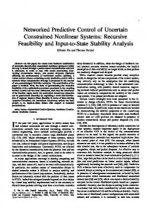
where Φk = e , Γk = 0 e R hk As e dsB . 2 0 Because the sampling period hk switches in the finite e k used in (4) also switch in finite sets. set ϑ; Φk , Γk and Γ Then, the problem of H∞ controller design for (1) can be reduced to the corresponding problem for (4). Remark 1. As shown in Fig. 1, the control input u k−3 does not reach the actuator at the instant tk−3 + d2 for a long time delay, the sensor will sample plant0 s state at tk−3 + d2 , and the delayed control input will be dropped. The control input u k−1 is dropped, and the sensor will also begin the next sampling at the instant tk−1 + d2 . The sampling begins only when the former sampled packet reaches or is dropped, so packet disordering cannot occur.
2
H ∞ controller design dropout compensation
with
815
packet
To compensate the packet dropout of NCSs, a linear estimator might be added into the system to estimate the dropped control input packets. Suppose the states x 0 , x k1 , x k2 , · · · , x kj , · · · , and the corresponding control inputs on the basis of these states are transferred to the actuator successfully, and suppose L − 1 is the maximum number of consecutive packets dropout. Then, the estimated values of the dropped control inputs are as follows. 1 1 ukj u k = (1 − )u L j L 2 ˆ kj +1 + (ˆ ukj ˆ kj +2 = u u u kj +1 − u kj ) = (1 − )u L 3 ˆ kj +3 = u ˆ kj +2 + (ˆ ˆ kj +1 ) = (1 − )u ukj u u kj +2 − u L ··· ˆ kj+1 −1 = u ˆ kj+1 −2 + (ˆ ˆ kj+1 −3 ) = u u kj+1 −2 − u kj+1 − kj − 1 ukj (1 − )u L ˆ kj +1 = u kj − u
(5)
where L is a predefined positive scalar. Without loss of generality, by supposing the disturbance inputs ω kj = ω kj +1 = · · · = ω kj+1 −1 for every kj and using the packet dropout compensation method given above, the evolution of plant states can be described as follows. eh ω k = ˆ kj −1 + Γ x kj +1 = Φhkj x kj + Γhkj u j kj kj − kj−1 − 1 eh ω k xkj−1 + Γ Φhkj x kj − (1 − )Γhkj Kx j kj L e bω k = x kj +2 = Φbx kj +1 + Γbu kj + Γ j eh + Γ e b )ω xkj + (Φb Γ ω kj − (Φb Φhkj − Γb K)x kj kj − kj−1 − 1 xkj−1 )Φb Γhkj Kx (1 − L e bω k = ˆ kj +1 + Γ x kj +3 = Φbx kj +2 + Γbu j 1 xkj − [Φb 2 Φhkj − Φb Γb K − (1 − )Γb K]x L kj − kj−1 − 1 2 xkj−1 + )Φb Γhkj Kx (1 − L 2e eb + Γ e b )ω ωk (Φb Γh + Φb Γ j
kj
···
ej x k + B ej x k e x kj+1 = A j j−1 + Dj ω kj Ahk
Fig. 1
Both clock-driven and event-driven sampling
Remark 2. To use the active-varying sampling period method, [d1 , d2 ] should be partitioned into l equidistant small intervals, and a large l can ensure the computational precision, but it might lead to frequent switching of sampling period, so l can be chosen on the basis of d2 − d1 . If d2 − d1 is large, l should be large, otherwise, l should be small. The following lemma will be used in the sequel. Lemma 1[7] . Suppose a ∈ Rn , b ∈ Rm , and G ∈ Rn×m . Then, for any X ∈ Rn×n , Y ∈ Rn×m , and Z ∈ Rm×m satisfying · ¸ X Y ≥0 YT Z the following inequality holds aT Gbb ≤ −2a
· ¸T · X a b Y T − GT
¸· ¸ Y −G a b Z
Ad2
R hkj
(6) As
where Φhkj = e , Φb = e , Γhkj = 0 e dsB1 , R hkj As R d2 As eb = e e dsB2 , Γb = e dsB1 , Γ Γhkj = 0 0 R d2 As e dsB2 , and 0 j
ej = Φb kj+1 −kj −1 Φh − Φb kj+1 −kj −2 Γb K− A kj 1 kj+1 −kj −3 (1 − )Φb Γb K− L 2 kj+1 −kj −4 (1 − )Φb Γb K − · · · − σ1 Γb K L kj+1 −kj −1 e Bj = −σ2 Φb Γh K kj
e j = Φb kj+1 −kj −1 Γ e h + Φb kj+1 −kj −2 Γ eb + · · · + Γ eb D kj kj+1 − kj − 2 ) σ1 = (1 − L kj − kj−1 − 1 σ2 = (1 − ) L
(7) Define x kj+1 , x kj , x kj−1 , and ω kj as ξ j+1 , ξ j , ξ j−1 , and ω j , respectively. Then, ej ξ + B ej ξ e ξ j+1 = A j j−1 + Dj ω j
(8)
816
ACTA AUTOMATICA SINICA Vol. 34 · ¸ X Y We are now in a position to design the feedback gain ≥ 0, we have YT Z K, which can make system (8) asymptotically stable with the H∞ norm bound γhkj (γhkj is the H∞ norm bound e e T e ξ −ξ −2 ξ T j (Aj + Bj ) P Bj (ξ j j−1 ) ≤ corresponding to the sampling period hkj ). T T T ej + B ej ) P B ej ](ξξ − ξ Theorem 1. If there exist symmetric positive definite ξ j Xξξ j + 2ξξ j [Y − (A j j−1 )+ e and Z, e and matrices X, e Ye , N , and scalars T matrices M , R, (ξξ j − ξ j−1 ) Z(ξξ j − ξ j−1 ) γhkj > 0, such that the following LMIs (9) and (10) hold (13) for every feasible values of kj+1 − kj and hkj (kj+1 − kj = ∆V2j = (ξξ j+1 − ξ j )T Z(ξξ j+1 − ξ j )− 1, · · · , L, hkj ∈ ϑ)
−Ye e −R ∗ ∗ ∗ ∗
Ψ0 ∗ ∗ ∗ ∗ ∗
M C1T −σ2 N T D1T 0 −γhkj I ∗ ∗
0 0 −γhkj I ∗ ∗ ∗ ·
e X Ye T
ΨT 1 ΨT 2 e jT D 0 −M ∗
¸ Ye e ≥0 Z
ΨT 1 −M ΨT 2 T e Dj