h, protocol parameters V and parameters of the network setup δ. Thus, the sampling period h affects the performance of both wireless network and control ...
1
Wireless Networked Control System Co-Design Pangun Park, Jos´e Ara´ujo and Karl Henrik Johansson
Abstract—A framework for the joint design of wireless network and controllers is proposed. Multiple control systems are considered where the sensor measurements are transmitted to the controller over the IEEE 802.15.4 protocol. The essential issues of wireless networked control systems (NCSs) are investigated to provide an abstraction of the wireless network for a co-design approach. We first present an analytical model of the packet loss probability and delay of a IEEE 802.15.4 network. Through optimal control techniques we derive the control cost as a function of the packet loss probability and delay. Simulation results show the feasible control performance. It is shown that the optimal traffic load is similar when the communication throughput or control cost are optimized. The co-design approach is based on a constrained optimization problem, for which the objective function is the energy consumption of the network and the constraints are the packet loss probability and delay, which are derived from the desired control cost. The co-design is illustrated through a numerical example.
Keywords: Co-design, Linear Quadratic Gaussian controller, Medium Access Control, IEEE 802.15.4, Optimization. I. I NTRODUCTION There are major advantages in terms of increased flexibility, reduced installation, and maintenance costs in the use of wireless communication technology in industrial control systems [1], [2]. The IEEE 802.15.4 standard has received considerable attention as a low data rate and low power protocol for wireless sensor network (WSN) applications in industrial control, home automation, and smart grids [1]–[3]. Although WSNs provide a great advantage for the process and manufacturing industries, they are not yet efficiently deployed. One of the most significant reasons is the lack of proper modeling of the network behavior. Any wireless network introduces random packet losses and delays due to the harsh nature of the wireless channel, limited bandwidth, and interference generated by other wireless devices. The tradeoff between tractability and accuracy of the analytical model of a wireless network is important in order to hide the system complexity through a suitable abstraction without losing critical aspects of the network. Furthermore, WSNs require energy-efficient operation due to the limited battery power of each sensor node. Design methods on how to achieve high performance of control systems through a communication network have been recently proposed. The approaches can be grouped in two categories: design of the control algorithm and design of the communication protocol. Some research has been done in designing robust controllers and estimators that are adaptive and robust to the communication faults: The authors are with the ACCESS Linnaeus Center, Electrical Engineering, Royal Institute of Technology, Stockholm, Sweden. E-mails: {pgpark,araujo,kallej}@ee.kth.se. The work of the authors was supported by the EU project FeedNetBack, the Swedish Research Council, the Swedish Strategic Research Foundation, and the Swedish Governmental Agency for Innovation Systems.
packet dropout as a Bernoulli random process [4] or with deterministic rate [5], packet delay [6], and data rate limitation [7]. On the other side, communication protocols and their parameters are designed in order to achieve a given control performance. In [8], the authors present a scheduling policy to minimize a linear quadratic (LQ) cost under computational delays. In [9], the authors proposed an adaptive tuning scheme of the parameters of the link layer, medium access control (MAC) layer and sampling period through numerical results in order to minimize the LQ cost. However, these approaches often consider only one aspect of the network faults: packet dropout [4],[5], packet delay [6], [8], or data rate limitation [7]. In [9], although the authors consider the simulation results of the wireless network, the framework has not been designed out of an analytical consideration of control performance. Even though many communication protocols are available in [10] and [11], these protocols are designed mainly to achieve high reliability and high energy efficiency for various applications of WSNs and not specifically for control applications. In this paper there are two original contributions: 1) We investigate the essential issues of wireless networked control systems (NCSs) by considering the effects of wireless network on control performance. 2) We propose a co-design approach to meet the desired control cost while minimizing the energy consumption of the network. In particular, we show the feasible control performance by considering the wireless network effects. This paper explicitly considers both the control cost of control applications and the network performance with respect to energy consumption, which is the most important requirement of communication protocol design for WSNs. The key issue addressed here is how to derive the explicit relation between the performance of the control systems and the characteristics of a wireless network. Furthermore, the well-defined design procedure is investigated to achieve high performances in wireless NCSs. The outline of the paper is as follows. Section II defines the considered problem of control over a wireless network. In Section III, we describe the IEEE 802.15.4 standard and its network model. The design of the estimator and the controllers is presented in Section IV. In Section V, we discuss the essential issues of wireless NCSs based on simulation results and propose a co-design approach. In Section VI, we illustrate it through numerical examples. Section VII concludes the paper. II. P ROBLEM F ORMULATION The problem considered is depicted in Fig. 1, where multiple plants are controlled over a WSN using the IEEE 802.15.4 protocol. M plants contend to transmit sensor measurements to the controller over a wireless network that induces packet
2
Packet loss is first modelled as a random process whose parameters are related to the behavior of the network. The measurement at the controller side is given by � Cxk + vk , γk = 1 , (3) yˆk = 0, γk = 0 ,
Plant 1
Sensor 1 Plant i Plant M Wireless network ( IEEE 802.15.4 )
Network manager
State feedback
where γk is a Bernoulli random variable with Pr(γ k = 1) = 1 − p, where p is the packet loss probability which models the packet loss between the sensor and the controller. By considering both the packet loss and delay induced by a wireless network, �we introduce �T an augmented discrete-time to analyze the system. The state variable zk = xk uk−1 augmented state space is
Estimator
Network model Controller 1 Controller i Controller M
Fig. 1. Overview of the networked control system setup. M plants need to be controlled by M controllers. The wireless network closes the loop from the sensor nodes to the controllers.
losses and varying delays. We assume that a sensor node is attached to each plant. A contention-based IEEE 802.15.4 protocol is used to determine which sensor node accesses the wireless channel. Throughout this paper we consider control applications where nodes asynchronously generate packets when a timer expiries. When a node sends a packet successfully or discards a packet, it stays in an idle period for h seconds without generating packets. The data packet transmission is successful if an acknowledgement (ACK) packet is received. We assume that the controller commands are always successfully received by the actuator. Many practical NCSs have several sensing channels, whereas the controllers are collocated with the actuators, as in heat, ventilation and airconditioning control systems [12]. We consider a plant i, for i = 1, . . . , M , given by a linear stochastic differential equation dx(t) = Ax(t)dt + Bu(t)dt + dw(t)
(1)
where x(t) ∈ Rn is the plant state and u(t) ∈ Rm is the control signal. The process disturbance w(t) ∈ R n has a mean value of zero and uncorrelated increments, with incremental covariance Rw dt. We neglect the plant index i to simplify notation. Let us consider the sampling of the plant with timevarying sampling period h k = tk+1 − tk and delay dk [13]. The sampling period is h k = h+ dk where the idle period h is constant and the random delay is d k , which is bounded d k ≤ dreq . We assume that the random sequences {d k } and {hk } are bounded, 0 < d k < hk and 0 < hmin ≤ hk ≤ hmax . In addition, they are independent and have known distributions. Notice that the networked induced delay d k is less than hk and allows the packets to arrive at the controller in the correct order. By considering zero-order-hold, a time-varying discretetime system is obtained Γk0 uk
xk+1 = Φk xk + yk = Cxk + vk
+
Γk1 uk−1
+ wk (2)
�� hk −dk
�
where Φk = eAhk , Γk0 = eAs ds B, Γk1 = 0 �� � hk eAs ds B, and vk is a discrete-time white Gaussian hk −dk noise with zero mean and variance R v . The parameter k is the discrete time index. The initial state x 0 is white Gaussian with mean x ¯0 and covariance P 0 .
zk+1 = Φd zk + Γd uk + wk yˆk = γk yk (4) � � � � Φ Γ1 Γ0 where Φd = , Γd = and Cd = C 0 . 0 0 I In Fig. 1, a network manager block is introduced to achieve an efficient control system over a wireless network. Particularly, the network manager requires an analytical model of the packet loss and delay (i.e., between the sensors and controller). Then, this model is used to design the estimator and controller that compensate for the packet loss and delay induced by the network. The network manager is based on a constrained optimization problem where the objective function, denoted by Etot , is the total energy consumption of the wireless network and the constraint is the desired control cost. Hence, the constrained optimization problem of the control system is min h,V
s.t.
Etot (h, V, δ)
(5a)
J(h, p(h, V, δ), d(h, V, δ)) ≤ Jreq .
(5b)
The decision variables are h, which is the sampling period, and V, which are the protocol parameters of the network. δ includes the parameters of the network setup such as a network topology, length of packet, and number of nodes. J(h, p(h, V, δ), d(h, V, δ)) is the control cost, which is a function of the sampling period h, packet loss probability p, and delay d of the network, and J req is the desired maximum control cost. We remark that the packet loss probability and delay of the network is also a function of the sampling period h, protocol parameters V and parameters of the network setup δ. Thus, the sampling period h affects the performance of both wireless network and control system. In (5b), the decision variables are feasible if they satisfy a given control cost J req . Note that it is possible to pose different optimization problems under the same framework. III. W IRELESS M EDIUM ACCESS C ONTROL P ROTOCOL In this section, we introduce the effective analytical model of packet loss probability and delay of the wireless network imposed by the IEEE 802.15.4 protocol which was originally derived in [14]. The contention-based MAC protocol of the IEEE 802.15.4 standard is used for control systems in this paper. We first present the overview of the carrier sense multiple access with collision avoidance (CSMA/CA) mechanism of the IEEE 802.15.4 protocol and provide an analytical model of the wireless network.
3
Consider a node trying to transmit. In the slotted CSMA/CA algorithm, first the MAC sub-layer of the node initializes four variables, i.e., the number of backoffs (NB=0), contention window (CW=2), backoff exponent (BE=macMinBE), and retransmission times (RT=0). Then the MAC sub-layer delays for a random number of complete backoff periods in the range [0, 2BE − 1] units. When the backoff period is zero, the node performs the first Clear Channel Assessment (CCA). If two consecutive CCAs are idle, then the node commences the packet transmission. If either of the CCA fails due to a busy channel, the MAC sublayer will increase the value of both NB and BE by one up to a maximum value macMaxCSMABackoffs and macMaxBE, respectively. Hence, the value of NB and BE depend on the number of CCA failures of a packet. Once the BE reaches macMaxBE, it remains at the value of macMaxBE until it is reset. If NB exceeds macMaxCSMABackoffs, then the packet is discarded due to the channel access failure. Otherwise, the CSMA/CA algorithm generates a random number of complete backoff periods and repeats the process. Here, the variable macMaxCSMABackoffs represents the maximum number of times the CSMA/CA algorithm is required to backoff. If channel access is successful, the node transmits the frame and waits for ACK. The reception of the corresponding ACK is interpreted as successful packet transmission. If the node fails to receive ACK due to collision or ACK timeout, the variable RT is increased by one unit up to macMaxFrameRetries units. If RT is less than macMaxFrameRetries, the MAC sublayer initializes two variables CW=0, BE=macMinBE and follows the CSMA/CA mechanism to re-access the channel. Otherwise the packet is discarded due to the retry limits. In such a scenario, a precise and effective analytical model of the slotted CSMA/CA of the IEEE 802.15.4 standard was proposed in [14]. It is modelled through a Markov chain taking into account retry limits, ACKs, unsaturated traffic load, and the parameters of the network setup such as a length of packet and number of nodes. Let s(t), c(t) and r(t) be the stochastic process representing the backoff stage, the state of the backoff counter, and the state of retransmission counter at time t, respectively, experienced by a node to transmit a packet. By assuming that nodes start sensing independently, the stationary probability μ that the node attempts the first carrier sensing in a randomly chosen slot time is constant and independent of the other nodes. It follows that (s, c, r) results in a three dimensional Markov chain with the time unit aUnitBackoffPeriod (corresponding to 0.32 ms). The channel accessing probability μ that a node attempts the first CCA, the first busy channel probability α for the first CCA, and the second busy channel probability β for the second CCA are derived by solving the state transition probabilities associated with the Markov chain model. Note that the expressions of μ, α, and β are computed by solving a system of non-linear equations. The precise model gives us the objective function, energy consumption (5a), and the packet loss probability and delay in a numerical form. Note that the protocol parameters V of the decision variables are the MAC parameters (macMinBE, macMaxCSMABackoffs, macMaxFrameRetries). IV. D ESIGN OF E STIMATOR AND C ONTROLLER In this section, we investigate how the packet loss probability and delay of the network affect the control performance.
We discuss the design of an optimal feedback controller and present a control cost to analyze the NCSs described in Section II. We first introduce our performance indicator as a control cost function, which is an explicit function of the sampling period h, packet loss probability p, and delay d of the network. Then, we design the estimator and controller under packet losses and delays in Section IV-A and IV-B, respectively. This is achieved by extending the results on optimal stochastic estimation and control under packet losses in [4] with delays in [6]. Let us first define the information set under the packet loss and network induced delay as follows Ik = {yk , γ k }
(6)
where yk = (yk , yk−1 , . . . , y1 ) and γ k = (γk , γk−1 , . . . , γ1 ). Consider the control cost function T JN (uN −1 , z¯0 , P0 ) = E[zN WN zN
+
N −1
(zkT Wk zk + 2zkT Nk uk + uTk Uk uk )],
(7)
k=0
�T � ¯0 0 , P0 is the covariance of the initial where z¯0 = x condition, and the matrices W k , Nk and Uk are time-invariant, symmetric and positive definite. In the following section, we introduce the estimator design. A. Estimator Design The estimator design is based on arguments similar to the standard Kalman filtering. Let us define the following variables �T � zˆk|k = E[xk |Ik ] uk−1 Pk|k = E[(zk − zˆk|k )(zk − zˆk|k )T |Ik ]. The innovation step is given by zˆk+1|k = Φd E[zk |Ik ] + Γd uk = Φd zˆk|k + Γd uk Pk+1|k =
Φd Pk|k ΦTd
+ Rw
(8) (9)
where wk and Ik are independent and u k is a deterministic function of I k . The correction step is given by zˆk+1|k+1 = zˆk+1|k + γk+1 Kk+1 (yk+1 − Cd zˆk+1|k )
(10)
−1
Pk+1|k CdT (Cd Pk+1|k CdT
Kk+1 = + Rv ) Pk+1|k+1 = Pk+1|k − γk+1 Kk+1 Cd Pk+1|k
(11)
where we apply the standard derivation for the Kalman filter. B. Controller Design We introduce the feedback control law and present the finite and infinite horizon control cost functions. The cost function given by Eq. (7) can be expressed as ∗ =V0 (x0 ) = z¯0T S0 z¯0 + Tr(S0 P0 ) + JN
N −1
(Tr((ΦTd Sk+1
k=0
× Φd + Wk − Sk )Eγ [Pk|k ]) + Tr(Sk+1 Rw ))
(12)
where Sk is the solution of the Riccati equation as defined in [4] and Tr denotes the trace of a square matrix. E γ [·] is
4
Jreq
Jreq
network
network
(a) Feasible control cost for the simplified case. (b) Feasible control cost with M = 10. (c) Feasible control cost with M = 20. Fig. 2. Feasible control cost over different sampling periods, packet loss probabilities, and packet delays. The colors show the control cost. Note that the scales of color bar are different in the figures.
the expectation with respect to the arrival sequence {γ k }. The control input that minimizes the cost function of Eq (7) is uk = −(ΓTd Sk+1 Γd + Uk )−1 ΓTd Sk+1 Φd zˆk|k = −Lk zˆk|k . (13) The expected value E γ [Pk|k ] is bounded by P˜k|k ≤ Eγ [Pk|k ] ≤ Pˆk|k ,
∀k ≥ 0
where the matrices P˜k|k and Pˆk|k can be found in [4]. Then, it is possible to derive the bound of control cost given in Eq. (12). min In the next section, we use two deterministic sequences J N max and JN , which bound the expected minimum cost as follows 1 ∗ 1 max 1 min JN ≤ JN ≤ JN , (14) N N N and the two sequences converge to the following values: max J∞ =Tr((ΦTd S∞ Φd + Wk − S∞ )(P ∞ − (1 − p)P ∞ CdT min J∞
× (Cd P ∞ CdT + Rv )−1 Cd P ∞ )) + Tr(S∞ Rw ) (15)
=pTr((ΦTd S∞ Φd + Wk − S∞ )P ∞ ) + Tr(S∞ Rw ) (16)
where, P ∞ =Φd P ∞ ΦTd + Rw − (1 − p)Φd P ∞ CdT × (Cd P ∞ CdT + Rv )−1 Cd P ∞ ΦTd
P ∞ =pΦd P ∞ ΦTd + Rw . We remark that Eqs. (15) and (16) are explicit functions of the sampling period h, packet loss probability p, and delay d. The finite horizon cost and the cost bounds of the infinite horizon case will be used as the performance indicators in Section V-A. V. C O -D ESIGN F RAMEWORK In this section, we first show the feasible control performance by taking into account realistic simulation results. Then, we study the co-design of the wireless NCS. A. Effects of Wireless Network In this section, we discuss the fundamental issues of codesign of communication network and controller for wireless NCSs. The control cost (15) is considered as a performance indicator of the control system as described in Section IV. As
an example we consider an unstable second-order plant in the form of (1) with � � � 3 1 0 1 0 A= , B= , C= , P0 = 0.01I 0 1 1 0 1 W = I, N = 0, U = 0.01, Rw = I, Rv = 0.01I, where W, N, U are assumed to be time-invariant in Eq. (7). Fig. 2 shows the feasible control cost with respect to different sampling periods, packet loss probabilities, packet delays with the simplified case and the realistic wireless networks for the different number of nodes M = 10, 20. Note that the simplified case does not explicitly consider the realistic network behavior i.e., independent relationship between sampling period, packet loss probability, and packet delay. In the figures, the colors show the feasible control cost. Fig. 2(a) depicts the simplified case where longer sampling periods increase the control cost. Furthermore, we observe that packet losses at a higher sampling period are more critical than packet losses at a lower sampling period, indicating that we are sampling in a conservative way. Similarly, we derive the effects of packet delay on the control cost. Figs 2(b) and 2(c) depict the feasible region for M = 10 and 20 nodes, respectively. Note that we set the desired control cost J req = 20. A point is feasible if it satisfies a given required cost, packet loss probability and delay for each sampling period. The feasible region is the set of all feasible points. In the figure, the transparent region denotes that the desired control cost is not feasible. It is natural that as the control requirement becomes strict, the infeasible region increases, since it also requires lower packet loss probability and delay of the network for lower sampling periods. Observe in Figs. 2(b) and 2(c) that the packet loss probability p ≤ 0.01 is not feasible when the sampling period is short h ≤ 0.03 s. Since short sampling periods increase the traffic load of the network, the packet loss probability is closer to the critical packet loss probability, above which the system is unstable. Hence, it is difficult to achieve a low packet loss probability when the sampling period is short. Furthermore, by comparing Figs. 2(b) and 2(c), we see that the infeasible region increases as the number of nodes increases. We remark that the infeasible region due to the wireless network starts from the origin where the sampling period h = 0, no packet loss p = 0, and no packet delay d = 0. No matter what communication protocol is used, the origin belongs to the infeasible region. The area and shape of the infeasible region depends on the communication protocol.
5
0.7
18 i J∞
∗ JN
14
control cost
0.65
r J∞
0.6
(2)
throughput
12
0.55
10
0.5
8
0.45
6
0.4
throughput
16
(1)
Setup network model and requirement Jreq
Tune Jreq (4) (3)
Solve constrained optimization according to (17) for different h .
No 0.35
0
L
S
2
0.3 0.25
(5)
Update estimator and state ∗ feedback according to h
(6)
Success
Jreq 4
∗
Choose h and optimize network resources V ∗
Compute estimator (8)–(11) and state feedback (13) according to Section IV
Fig. 4.
Feasibility ?
Yes
Flow diagram of co-design framework.
greater than the minimum value of the control cost. Then, we have two feasible sampling periods S and L in Fig. 3. Fig. 3. Control cost and throughput of the wireless network over different However, the performance of the wireless network is still i r max sampling periods. J∞ and J∞ refer to the cost bound J∞ of the infinite horizon control cost given in (15) with ideal case and realistic model in [14], heavily affected by the choice of the sampling period of S and ∗ denotes the finite horizon control cost given in (12). respectively. JN L, as we discussed earlier. By choosing L, the throughput of the network is stabilized (see details in [15]), hence, the control Fig. 3 shows the control cost and communication throughput cost is also stabilized with respect to small perturbations over different sampling periods. The throughput is the average of the network. Therefore, the wireless NCSs achieve good rate of successful data transmission over a communication robustness for both communication and control perspective by channel, which is the common objective for a communication choosing L. Furthermore, a longer sampling period L leads to i r and J∞ refers to the cost bound lower network energy consumption than the shorter sampling designer. In the figure, J ∞ max J∞ given by Eq. (15) for the ideal (no packet loss and no period S in [14]. Recall that the energy efficiency is one of ∗ the most critical issues for sensor nodes due to their limited delay) and realistic model in [14], respectively. Recall that J N is the finite horizon control cost given by Eq. (12). The cost battery power. This motivates our co-design approach of NCSs ∗ r JN follows the infinite horizon cost J ∞ based on the realistic running over WSNs. model. Due to the absence of packet losses and delays, the control performance when using an ideal network increases B. Design Procedure monotonically as the sampling period increases. However, We remind that the problem we consider in this paper is when using a real network, a shorter sampling period does not how to determine the optimal sampling period h ∗ of control minimize the control cost of the control systems, because of systems and the protocol parameters V ∗ of the communication the higher packet loss probability when the traffic load is high. protocol of an optimization problem given by Eq. (5). Fig. 4 i r and J∞ coincide shows the proposed design flow that each control loop of In addition, the two curves of the cost J ∞ for longer sampling periods, meaning that when the sampling the network follows. The application designer provides the period is larger, the sampling period is the dominant factor in parameters of network setup δ and the desired maximum the control cost compared to the packet loss probability and control cost Jreq . δ includes the important factors for modeling delay. the wireless network such as a network topology, length of the Now, let us discuss the throughput of the communication packets, and the number of nodes (step 1). It is also possible network and control cost of control systems. When we flip the that each control loop has a different desired maximum control throughput curve on the Y-axis, we observe a similar trend of cost Jreq . The control designer then computes, off-line, an behavior with the curve of control cost. Note that the closer estimator (8)–(11) and a state feedback (13) according to the throughput is to 1, the better the utility of the wireless Section IV for different sampling periods, packet loss probanetwork. As the sampling period h ∈ [0, 0.13] s increases, bilities, and delays (step 2). The network manager formulates the control cost decreases and the throughput increases due and solves a constrained optimization problem, whereby the to mainly high packet loss. For a longer sampling period objective function is the energy consumption of the network h > 0.15 s, the performance of both the communication and and the constraints are the packet loss probability and delay, control system degrades as the sampling period increases. The which are derived from J req for different sampling periods throughput decreases since the network is underutilized. We (step 3). More precisely, the constrained optimization problem remark that the objective of both communication design and is formulated from (5) for a given sampling period h as follows control design has a very similar trend. Hence, the optimal min Etot (h, V, δ) (17a) traffic load of the network is similar when the communication V throughput or control cost are optimized. Even though the (17b) s.t. p(h, V, δ) ≤ preq , dynamic interactions between these two objectives, throughput d(h, V, δ) ≤ dreq . (17c) of the communication and control cost of control system, are critical factors for wireless NCSs, these issues are not well The decision variables are the communication protocol paraminvestigated in the previous literatures. eters V depending on the network designer. The adaptive IEEE Let us consider a desired maximum control cost J req 802.15.4 protocol [16] is applied to meet the requirements for 0.05
0.1
0.15
0.2
sampling period (s)
0.25
0.3
6 0.8
12
0.7
10
1000
0.04
900
0.035
800
0.03
0.6 8
700 0.025 0.5
600
0.4
500
6
0.02 0.015
4
400 0.3
0.01
300 2
0
0.2
0
100
200
300
time (s)
400
500
600
0.1
0.005
200
0
100
200
300
time (s)
400
500
600
100
0
100
200
300
time (s)
400
500
600
0
0
100
200
300
time (s)
400
500
600
(a) control cost. (b) power consumption of a node. (c) interval of packet generated time. (d) packet loss probability. Fig. 5. Optimized control cost, power consumption of the network, interval of packet generated time, and packet loss probability of the proposed co-design approach with M = 20 nodes when the control requirement changes from Jreq = 11 to Jreq = 3 at 315 s. The particular realization is shown out of M = 20 nodes. The dotted line shows the requirement change of each figures.
packet loss probability and packet delay for a given sampling period. One can find a sub-optimal solution using the steps described in [16]. The network manager finds the local optimal MAC parameters V∗ (h, preq , dreq ) of a sub-optimization problem for a given h, p req , dreq . Then, the optimal solution h ∗ , V∗ is given by the pair h, V that minimizes the cost function if there are feasible solutions (step 5). Otherwise, the control designer needs to tune J req since the desired control cost is not realistic (step 4). The network manager adapts the optimal sampling period h ∗ and the optimal protocol parameters V ∗ of the network (step 5). The control designer updates the estimator and the state feedback according to the optimized h∗ , p(h∗ , V∗ , δ), d(h∗ , V∗ , δ) (step 6). VI. I LLUSTRATIVE E XAMPLE In this section, we illustrate the proposed co-design procedure described in Section V-B through numerical examples. Fig. 5 shows the adaptation of the requirements in terms of the sampling period, and packet loss probability of the network when the control requirement changes from J req = 11 to Jreq = 3 at 315 s. The optimal parameters h ∗ , preq , dreq are 214.4 ms, 0.012, 74.9 ms before control requirement changes, respectively. Figs. 5(c), and 5(d) show that the adaptive communication protocol satisfies the requirements of h and preq , respectively. Note that the proposed protocol also meets the requirement of the packet delay. The high jitter of Fig. 5(c) is mainly due to the packet loss of Fig. 5(d). After the control requirement changes at time 315 s, the optimal parameters h, preq , dreq adapt to 102.4 ms, 0.037, 97.4 ms, respectively. We remark that although the requirements of packet loss probability and packet delay are less strict after the requirement changes, the sampling period decreases to meet the requirement Jreq = 3. Recall that as the sampling period decreases, the packet loss probability and packet delay increase. Observe that the control cost is satisfied and the convergence of the algorithm is very fast. By comparing Figs. 5(a) and 5(b), the tradeoff between the control cost and power consumption of the network is clearly observed. VII. C ONCLUSIONS The dynamic interactions between communication network and control system are critical factors to guarantee the stability of wireless NCS. In this paper, it is shown how the design framework of the WSNs is applicable to control applications. We first present how the wireless network affects the performance of NCSs by showing the feasible region of the control performance. Furthermore, the optimal traffic load of the network is similar when the communication throughput or control cost are optimized. By considering these results, we conclude
that the sampling period significantly influences not only the control performance, and throughput and energy consumption of the network, but also the robustness of the wireless NCS. A co-design between communication and control application layers is proposed for multiple control systems over the IEEE 802.15.4 wireless network. In particular, a constrained optimization problem is studied, where the objective function is the energy consumption of the network and the constraints are the packet loss probability and delay, which are derived from the desired control cost. Numerical results illustrate the efficiency of the proposed co-design approach. R EFERENCES [1] A. Willig, “Recent and emerging topics in wireless industrial communication,” IEEE Transactions on Industrial Informatics, vol. 4, no. 2, pp. 102–124, 2008. [2] P. Park, “Protocol design for control applications using wireless sensor networks,” KTH, Tech. Rep., 2009, http://www.ee.kth.se/∼ pgpark/ papers/TRITA-EE-200904.pdf. [3] IEEE 802.15.4 standard: Wireless Medium Access Control and Physical Layer Specifications for Low-Rate Wireless Personal Area Networks, IEEE, 2006, http://www.ieee802.org/15/pub/TG4.html. [4] L. Schenato, B. Sinopoli, M. Franceschetti, K. Poola, and S. Sastry, “Foundations of control and estimation over lossy networks,” Proceedings of the IEEE, vol. 95, no. 1, pp. 163–187, 2007. [5] M. Yu, L. Wang, G. Xie, and T. Chu, “Stabilization of networked control systems with data packet droupout via switched system approach,” in IEEE CACSD, 2004. [6] J. Nilsson, “Real-time control systems with delays,” Ph.D. dissertation, Lund Institute of Technology, 1998. [7] G. N. Nair, F. Fagnani, S. Zampieri, and R. J. Evans, “Feedback control under data rate constraints: An overview,” Proceedings of the IEEE, vol. 95, no. 1, pp. 108–137, 2007. [8] D. Henriksson and A. Cervin, “Optimal on-line sampling period assignment for real-time control tasks based on plant state information,” in IEEE CDC, 2005. [9] X. Liu and A. J. Goldsmith, “Wireless network design for distributed control,” in IEEE CDC, 2004. [10] J. N. Al-Karaki and A. E. Kamal, “Routing techniques in wireless sensor networks: a survey,” IEEE Transactions on Wireless Communications, vol. 11, no. 6, pp. 6–28, 2004. [11] A. Bachir, M. Dohler, T. Watteyne, and K. K. Leung, “MAC essentials for wireless sensor networks,” IEEE Communications Surveys and Tutorials, vol. 12, no. 2, pp. 222–248, 2010. [12] T. Arampatzis, J. Lygeros, and S. Manesis, “A survey of applications of wireless sensors and wireless sensor networks,” in IEEE MCCA, 2005. [13] K. J. Astr¨om and B. Wittenmark, Computer-Controlled Systems. Prentice Hall, 1997. [14] P. Park, P. D. Marco, P. Soldati, C. Fischione, and K. H. Johansson, “A generalized Markov chain model for effective analysis of slotted IEEE 802.15.4,” in IEEE MASS, 2009. [15] R. Rom and M. Sidi, Multiple access protocols: performance and analysis. Springer-Verlag, 1990. [16] P. Park, , C. Fischione, and K. H. Johansson, “Adaptive IEEE 802.15.4 protocol for energy efficient, reliable and timely communications,” in ACM/IEEE IPSN, 2010.