Half-Against-Half Multi-class Support Vector Machines Hansheng Lei
[email protected]
Venu Govindaraju
[email protected]
CUBS, Center for Biometrics and Sensors Department of Computer Science and Engineering State University of New York at Buffalo Amherst, NY 14260-2000, USA Editor: ***
Abstract A Half-Against-Half (HAH) multi-class SVM is proposed in this paper. Unlike the commonly used One-Against-All (OVA) and One-Against-One (OVO) implementation methods, HAH is built via recursively dividing the training dataset of K classes into two subsets of classes. The structure of HAH is same as a decision tree with each node as a binary SVM classifier that tells a testing sample belongs to one group of classes or the other. The trained HAH classifier model consists of at most 2dlog2 (K)e binary SVMs. For each classification testing, HAH requires at most dlog2 (K)e binary SVM evaluations. Both theoretical estimation and experimental results show that HAH has advantages over OVA and OVO based methods in the testing speed as well as the size of the classifier model while maintaining comparable accuracy. Keywords: Multi-class classification, Support Vector Machines, Half-Against-Half
1. Introduction Support Vector Machine (SVM) has been proved to be a fruitful learning machine, especially for classification. Since it was originally designed for binary classification (Boser et al. (1992)), it is not a straightforward issue to extend binary SVM to multi-class problem. Constructing K-class SVMs (K À 2) is an on-going research issue (Allwein et al. (2000), Bredensteiner and Bennet (1999)). Basically, there are two types of approaches for multi-class SVM. One is considering all data in one optimization (Crammer and Singer (2001)). The other is decomposing multiclass into a series of binary SVMs, such as ”One-Against-All” (OVA) (Vapnik (1998)), ”One-Against-One” (OVO) (Kreßel (1999)), and DAG (Platt et al. (2000). Although more sophisticated approaches for multi-class SVM exist, extensive experiments have shown that OVA, OVO and DAG are among the most suitable methods for practical use (Hsu and Lin (2002), Rifin and Klautau (2004)). OVA is probably the earliest approach for multi-class SVM. For K-class problem, it constructs K binary SVMs. The ith SVM is trained with all the samples from the ith class against all the samples from the rest classes. Given a sample x to classify, all the K SVMs are evaluated and the label of the class that has the largest value of the decision function 1
is chosen: class of x = argmaxi=1,2,...,K (wi · x + bi ),
(1)
where wi and bi depict the hyperplane of the ith SVM. OVO is constructed by training binary SVMs between pairwise classes. Thus, OVO binary SVMs for K-class problem. Each of the K(K−1) SVMs model consists of K(K−1) 2 2 casts one vote for its favored class, and finally the class with most votes wins (Kreßel (1999)). DAG does the same training as OVO. During testing, DAG uses a Directed Acyclic Graph (DAG) architecture to make a decision. The idea of DAG is easy to implement. Create a list of class labels L = (1, 2, · · · , K) (the order of the labels actually does not matter). When a testing sample is given for testing, DAG first evaluates this sample with the binary SVM that corresponds to the first and last element in list L. If the classifier prefers one of the two classes, the other one is eliminated from the list. Each time, a class label is excluded. Thus, after K − 1 binary SVM evaluations, the last label remaining in the list is the answer. None of the three implementation methods above, OVA, OVO or DAG, significantly outperforms the others in term of classification accuracy. The difference mainly lies in the training time, testing speed and the size of the trained classifier model. Although OVA only requires K binary SVM, its training is most computationally expensive because each binary SVM is optimized on all the N training samples (suppose the training dataset has N binary SVMs to train, which sounds much samples altogether). OVO or DAG has K(K−1) 2 more than what OVA needs. However, each SVM is trained on 2N K samples. The overall training speed is significantly faster than OVA. For testing, DAG is fastest in that it needs only K − 1 binary SVM evaluation and every SVM is much smaller than those trained by OVA. As for the total size of classifier model, OVO is the most compact one since it has much less total number of support vectors than OVA has. DAG needs extra data structure to index the binary SVMs, thus, it is a little bit larger than OVO. Our motivation here is whether there potentially lurks different but competitive multiclass SVM implementation method? Fortunately, OVA, OVO and DAG are not the end of the story. In this paper, we will study a Half-Against-Half (HAH) multi-class SVM method. We compare it with OVA, OVO and DAG in several aspects, including the training and testing speed, the compactness of the classifier model and the accuracy of classification. The rest of this paper is organized as follows. In section 2, we describe the implementation of HAH. In section 3, we discuss related works and compare HAH with OVA, OVO and DAG via theoretical analysis and empirical estimation. Then, experiments are designed and discussed in section 4. Finally, conclusion is drawn in section 5.
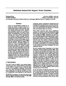
2. Half-Against-Half multi-class SVM Our motivation came from when we dealt with the classification problem of the Synthetic Control Chart (Scc) sequences (Hettich and Bay (1999)). Scc was synthetically generated to test the accuracy of time series classification algorithms. It has six different classes of control charts with 100 instances each class. Fig.1 shows examples of the Scc sequences. The existing multi-class SVMs all try to match one class against one another. This leads to OVA, OVO or DAG implementation method. Now, since the sequences in the last three classes are some kind of similar to each other, as shown in fig.1 D-F, can we 2
A. Normal
B. Cyclic
D. Decreasing trend
C. Increasing trend
F. Downward shift
E. Upward shift
Figure 1: Examples of the Scc sequences. There all 6 classes together. Class D,E and F have some kind similarity to each other.
A vs BC
DE vs F
A
AA AAAA A AA A
F B vs C
B
C C C C C C C CC C
B B B B B B B BB B
ABC vs DEF
DD DDDD D DD D
D vs E
C
D
F F F F F F F FF F
E
1)
E E E E E E E EE E
2)
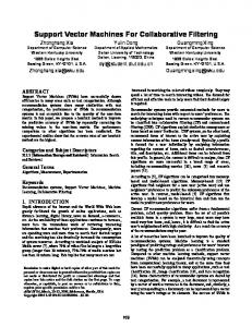
Figure 2: A possible decision tree for classifying the Scc samples. 1) Each node is a binary SVM that evaluates one group of classes against another group. 2) Half-AgainstHalf divisions of the six classes.
group them together as a bigger category {D,E,F} and match it against {A,B,C}? After a test sample is decided to lie in {D,E,F}, we can go further to see which class it should be labeled exactly. In this way, we have a recursive binary classification problem, which of course can be implemented by regular SVM. The structure of the classifier is same as a decision tree with each node as binary SVM. The classification procedure goes from root to the leaf guided by the binary SVMs, same as traveling a decision tree. Fig. 2 shows a possible SVM decision tree for the Scc data and the intuitive divisions of the 6 classes by Half-Against-Half. In the input space, two groups of classes might be nonseparable, but in the feature space, SVM can achieve good separation by kernel tricks. 3
1st level
ABDF vs CE
2nd level
AB vs DF
C vs E
C
3rd level A vs B
A
B
F
D
C
E
A
1)
E
D vs F
B
F
D
2)
Figure 3: The decision tree of HAH can follows the structure of the hierarchy clustering of the classes. 1) The hierarchy structure of the Scc dataset based on the mean distance between classes. 2)The corresponding decision tree of HAH.
For datasets with small number of classes, we can divide them into groups from coarse to fine manually with prior knowledge. Similar or close classes can be grouped together. Given a large K-class problem, its preferred to define groups automatically. Straightforwardly, we can recursively divide the K classes into two groups by random. The problem here is the separability between the arbitrary two groups might be not high, thus, the accuracy of classification is not reliable. The most desirable choice is to find the optimum two groups that lead to minimum expected error. With binary SVM, the expected error is E(error) = nSV N , where nSV is the number of support vectors (SV) and N is the number of training samples. Thus, the problem is equivalent to dividing classes into two halves with bK/2c which the trained SVM has the minimum number of SVs. For K classes, there are (K ) possible divisions. Training a binary SVM on each possible division and choosing the one with minimum nSV is not feasible. Unlike ”One-Against-One” and ”One-Against-All”, the dividing method is actually ”Half-Against-Half”. The biggest challenge is to determine the optimum divisions. While keeping the optimal division as an open problem, we found hierarchy clustering of classes is a suboptimal choice. Each class is considered as an element. The distance between two elements is defined as the mean distance between the training samples from the two classes. In this way, a hierarchy clustering structure for the K classes can be built. Then, the HAH model can be trained accordingly. Fig. 3 shows an example on the Scc dataset. The hierarchy of the 6 classes has dlog2 (6)e = 3 levels. Therefore, the corresponding decision tree of HAH has 3 levels.
3. Related works and Discussion A multistage SVM (MSVM) for multi-class problem was proposed in (Liu et al. (2003)). It uses Support Vector Clustering (SVC) (Ben-Hur et al. (2001)) to divide the training data into two parts and then a binary SVM is trained. For each part, the same procedure recursively takes place until the binary SVM gives a exact label of class. The unsolved 4
problem for MSVM is how to control the SVC to divide the training dataset into exact two parts. The two parameters, q (the scale of the Gaussian kernel) and C (the soft margin constant) could be adjusted to achieve this goal. However, this procedure is painful and unfeasible, especially for large datasets. The training set from one class could lie in both clusters. Moreover, there is no guarantee that exact two clusters can be found by varying p or C. HAH is an feasible solution for multi-class SVM. Compared with the OVA, OVO and DAG, HAH as its advantages. Table 1 summarizes the properties of the four methods. The structure of HAH is a decision tree with each node as a binary SVMs. The depth of the tree is dlog2 (K)e, therefore, the total number of nodes is 2dlog2 (K)e − 1. The training of DAG is same as OVO and both need to train K(K−1) binary SVMs. OVA has a binary SVMs for 2 each class, thus, it has K SVMs in total. The training time is estimated empirically by a power law (Platt (1999)): T ≈ αN 2 , where N is the number of training samples and α is some proportionality constant. Following this law, the estimated training time for OVA is: TOV A ≈ KαN 2
(2)
Without loss of generality, let’s assume the each of the K classes has the same number of training samples. Thus, each binary SVM of OVO only requires 2N K samples. The training time for OVO is: K(K − 1) 2N 2 ( ) ≈ 2αN 2 (3) TOV O ≈ α 2 K The training time for DAG is same as OVO. As for HAH, the training time is summed over all the nodes in the dlog2 (K)e levels . N In the ith level, there are 2i−1 nodes and each node uses 2i−1 training samples. Hence, the total training time is: dlog2 (K)e
THAH ≈
X i=1
α2i−1 (
N 2 ) ≈ 2i−1
dlog2 (K)e
X i=1
α
N2 ≈ 2αN 2 2i−1
(4)
Here, we have to notice that THAH does not include the time to build the hierarchy structure of the K classes, since doing so won’t consume much time and the quadratic optimization time dominates the total SVM training time. According the empirical estimation above, we can see that the training speed of HAH is comparable with OVA, OVO and DAG. In testing, DAG is faster than OVO and OVA, since it requires only K − 1 binary SVM evaluations. HAH is even faster than DAG because the depth of the HAH decision tree is dlog2 (K)e at most, which is superior to K − 1 especially when K À 2. Although the total number of SVs that do inner product with the testing sample contribute a major part of the evaluation time, the number of binary SVMs also counts. Our experiments also show that HAH has less kernel evaluations than DAG. The size of the trained classifier model is also an important concern in practical applications. The classifier model usually stay in the memory. Large model consumes a great portion of computing resources. The fourth column in table 1 is a coarse estimation of the size of model. Assume for each binary SVM, a portion of β of the training samples will become SVs. Since the number of SVs dominates the size, we can estimate the size of HAH is: 5
Table 1: The properties of HAH, OVO, DAG and OVA in training and testing. Method HAH DAG OVO OVA
Training # of SVMs Estimated Time 2dlog2 (K)e − 1 2αN 2 K(K − 1)/2 2αN 2 K(K − 1)/2 2αN 2 K KαN 2
Testing # of SVMs Size of Model dlog2 (K)e dlog2 (K)eβN K −1 (K − 1)βN K(K − 1)/2 (K − 1)βN K KβN
Table 2: Description of the multi-class datasets used in the experiments. Name Iris Scc PenDigits Isolet
# of Training Samples 105 420 7493 6238
dlog2 (K)e
SHAH ≈
X
i−1
2
i=1
# of Testing Samples 35 180 3497 1559
N (β i−1 ) ≈ 2
# of Classes 3 6 10 26
# of Attributes 4 60 16 617
dlog2 (K)e
X
βN = dlog2 (K)eβN
(5)
i=1
The size of OVO is: SOV O ≈
K(K − 1) 2N β = (K − 1)βN 2 K
(6)
The size of DAG is similar as OVO besides some extra data structure for easy indexing. Similarly, the size of OVA is estimated as KβN . According to the estimation above, HAH has the minimum size of classifier model among the four methods. Of course, real experiments are needed to testify the estimation.
4. Experiments According to the empirical estimation, HAH is superior to OVO, DAG and OVA in testing time and the size of classifier model. Experiments were conducted to firm this. Another very important concern is the classification accuracy. HAH was evaluated on multi-class datasets to compare its accuracy with that of OVO, DAG and OVA. The four datasets we used in experiments are: the Iris, the Scc,the PenDigits and the Isolet, all of which are from the UCI machine learning repository (Hettich and Bay (1999)). The description of the datasets are summarized in table 2. The Iris is one of the most classical datasets for testing classification. It has 150 instances (50 in each of three classes). The Scc dataset has 600 instances together (100 in each class). For both Iris and Scc, 70% were used as training samples, and the left 30% for testing. The PenDigits and Isolet were originally divided into training and testing subsets by the data donators. So, no change was made. On each dataset, we trained HAH, OVO, DAG and OVA based on the software LIBSVM (C.Chang and Lin (2001)) with some modification and adjustment. The kernel we chose was the RBF kernel, since it has been widely observed RBF kernel usually outperforms 6
Table 3: Experimental results by C-SVM.
Iris HAH OVO DAG OVA Scc HAH OVO DAG OVA PenDigits HAH OVO DAG OVA Isolet HAH OVO DAG OVA
σ
C
# of Kernel Evaluations
Size of Classifier Model (KByte)
Classification Accuracy
200 200 200 200
500 500 500 500
12 17 13 45
2.2 2.7 2.7 3.4
100% 100% 100% 100%
104 104 104 104
5 10 10 5
66 168 85 493
78.1 87.7 93.8 98.5
99.44% 99.44% 99.44% 99.44%
2 2 2 2
10 5 5 5
399 913 439 1927
183.9 300.0 305.0 223.1
98.37% 98.48% 98.43% 97.74%
200 200 200 200
5 10 10 5
935 3359 1413 6370
14,027 17,254 17,607 21,508
95.64% 96.60% 96.73% 94.23%
other kernels, such as linear and polynomial ones. The regularizing parameters C and σ were determined via cross validation on the training set. The validation performance was measured by training on 70% of the training set and testing on the left 30%. The C and σ that lead to best accuracy were selected. We also tried the ν-SVM for each method (Sch¨olkopf et al. (2000)). Similarly, a pair of ν and σ were chosen according to the best validation performance. We did not scale the original samples to range [-1,1], because we found that doing so did not help much. HAH was trained according to the hierarchy structure of the classes. Each class was considered as whole and the mean distance between two classes was used to build the hierarchy structure. OVO was implemented by the LIBSVM directly and thus we did not do any change. The DAG and OVA were also quite simple in implementation by modifying the LIBSVM source codes. The experimental results are summarized in table 3 and 4 by C-SVM and ν-SVM respectively. To compare HAH with OVO, DAG and OVA, three measures were recorded: i)Number of kernel evaluations, ii)Size of trained classifier model and iii)Classification accuracy. The number of kernel evaluations is the total number of support vectors that do kernel dot product with a single test sample. For OVO and OVA, all the support vectors need to do kernel evaluations with a given test sample. For HAH and DAG, different test samples may travel different pathes through the decision tree. So, we averaged the number of kernel evaluations over all testing samples. The number of kernel evaluations indicates the total testing CPU time. We used the kernel evaluations instead of the real testing CPU time because of implementation bias, i.e., the source codes on the same algorithm vary across 7
Table 4: Experimental results by ν-SVM.
Iris HAH OVO DAG OVA Scc HAH OVO DAG OVA PenDigits HAH OVO DAG OVA Isolet HAH OVO DAG OVA
σ
ν
# of Kernel Evaluations
Size of Classifier Model (KByte)
Classification Accuracy
200 200 200 200
0.05 0.05 0.05 0.10
9 8 7 35
1.9 2.3 2.3 3.0
100% 100% 100% 100%
103 103 103 103
0.015 0.05 0.05 0.015
103 254 204 1270
75.9 132.4 146.0 184.2
99.44% 99.44% 99.44% 98.33%
2 2 2 2
0.01 0.05 0.01 0.015
311 1464 353 2631
152.5 480.8 489.7 300.6
98.17% 97.91% 97.31% 97.37%
200 200 200 200
0.01 0.10 0.01 0.01
658 3520 760 5075
9,997 18,082 18,591 25,105
95.25% 96.54% 92.69% 93.97%
different programmers. The size of trained classifier model is a good measure how the classifier machine consumes computing resources. In real application with limited memory, such as online handwriting recognition in Personal Digital Assistants (PDAs), compact classifier model is desired. Accuracy, of course, is also very important for a classifier. Experimental results in both table 3 and 4 show that HAH has much less number of kernel evaluations than OVO and OVA. Since kernel evaluations dominates the testing time, HAH is much faster than OVO and OVA. As indicated by the number of kernel evaluations in both table 3 and table 4, HAH is between a factor of 2 to 5.3 times faster than OVO on the datasets PenDigits and Isolet, and 4 to 7.7 times faster than OVA. HAH is also faster than DAG, though not that significantly. HAH also has advantages over other methods in the compactness of the classifier model. The size of trained HAH model is around 1.7 to 3 times smaller than OVO and DAG, and about 2 to 2.7 times smaller than OVA. The datasets Iris and Scc are too small to show the advantages of HAH in both the testing speed and the compactness of model. However, they show that HAH can reach the same accuracy as OVO, DAG and OVA do. The accuracies on all the four datasets show that HAH is competitive with OVO, DAG and OVA. On dataset Isolet, the accuracy of HAH is about 1% lower than OVO but over 1% higher than DAG and OVA, as indicated by table 4. Considering HAH is 5.3 (3520/658) times faster than OVO in testing speed and 1.8 (18,082/9,997) times smaller in the size of model, the sacrifice of 1% accuracy is worthy. The reason why HAH is about 1% lower in accuracy over datasets with large number of categories like Isolet deserve further exploratory research. Dividing the classes into two groups optimally remains as an open problem. 8
5. Conclusions A Half-Against-Half multi-class SVM is proposed and studied in this paper. HAH has its advantages over commonly-used methods like OVO, DAG and OVA in the testing speed and the compactness of classifier model. The accuracy of HAH is also comparable with OVO, DAG and OVA. Further research on recursively dividing the classes into two groups optimally might improve the accuracy.
References E. Allwein, R. Schapire, and Y.Singer. Reducing multiclass to binary: A unifying approach for margin classifiers. In Machine Learning: Proceedings of the Seventeenth International Conference, 2000. A. Ben-Hur, D. Horn, H. Siegelmann, and V. Vapnik. Support vector clustering. Journal of Machine Learning Research, vol. 2:125–137, 2001. B. Boser, I.Guyon, and V. Vapnik. A training algorithm for optimal margin classifiers. In D. Haussler, editor, 5th Annual ACM Workshop on COLT, pages 144–152, 1992. E. Bredensteiner and K. Bennet. Multicategory classification by support vector machines. In Computational Optimizations and Applications, volume 12, pages 53–79, 1999. C.Chang and C. Lin. Libsvm: a library for support vector machines. http://www.csie.ntu.edu.tw/ cjlin/libsvm.
2001.
URL
K. Crammer and Y. Singer. On the algorithmic implementation of multiclass kernel-based vector machines. Journal of Machine Learning Research, vol. 2:265–292, 2001. S. Hettich and S. Bay. The UCI KDD archive. 1999. URL http://kdd.ics.uci.edu. C. Hsu and C. Lin. A comparison of methods for multi-class support vector machines. IEEE Transactions on Neural Networks, 13:415–425, 2002. U. Kreßel. Pairwise classification and support vector machines. In Advances in Kernel Methods: Support Vector Learnings, pages 255–268, Cambridge, MA, 1999. MIT Press. X. Liu, H. Xing, and X. Wang. A multistage support vector machine. In The 2nd International Conference on Machine Learning and Cybernetics, pages 1305–1308, 2003. J. Platt. Fast training of support vector machines using sequential minimal optimization. In Advances in Kernel Methods - Support Vector Learning, pages 185–208, Cambridge, MA, 1999. MIT Press. J. Platt, N. Cristianini, and J. Shawe-Taylor. Large margin DAGs for multiclass classification. In Advances in Neural Information Processing Systems, volume 12, pages 547–553, 2000. R. Rifin and A. Klautau. In defense of one vs-all-classification. Journal of Machine Learning Research, vol. 5:101–141, 2004. 9
B. Sch¨olkopf, A. Smola, R. Williamson, and P. Bartlett. New support vector algorithms. Neural Computation, 12:1207C1245, 2000. V. Vapnik. Statistical Learning Theory. Wiley, New York, 1998.
10