Predicting Tunnel Squeezing Using Multiclass Support Vector Machines

Hindawi Advances in Civil Engineering Volume 2018, Article ID 4543984, 12 pages https://doi.org/10.1155/2018/4543984

Research Article Predicting Tunnel Squeezing Using Multiclass Support Vector Machines Yang Sun, Xianda Feng , and Lingqiang Yang School of Civil Engineering and Architecture, University of Jinan, No. 336, West Road of Nan Xinzhuang, Jinan, Shandong 250022, China Correspondence should be addressed to Xianda Feng; [email protected] Received 13 December 2017; Revised 6 April 2018; Accepted 18 April 2018; Published 16 May 2018 Academic Editor: Carlos Chastre Copyright © 2018 Yang Sun et al. This is an open access article distributed under the Creative Commons Attribution License, which permits unrestricted use, distribution, and reproduction in any medium, provided the original work is properly cited. Tunnel squeezing is one of the major geological disasters that often occur during the construction of tunnels in weak rock masses subjected to high in situ stresses. It could cause shield jamming, budget overruns, and construction delays and could even lead to tunnel instability and casualties. Therefore, accurate prediction or identification of tunnel squeezing is extremely important in the design and construction of tunnels. This study presents a modified application of a multiclass support vector machine (SVM) to predict tunnel squeezing based on four parameters, that is, diameter (D), buried depth (H), support stiffness (K), and rock tunneling quality index (Q). We compiled a database from the literature, including 117 case histories obtained from different countries such as India, Nepal, and Bhutan, to train the multiclass SVM model. The proposed model was validated using 8-fold cross validation, and the average error percentage was approximately 11.87%. Compared with existing approaches, the proposed multiclass SVM model yields a better performance in predictive accuracy. More importantly, one could estimate the severity of potential squeezing problems based on the predicted squeezing categories/classes.

1. Introduction Redistributed stresses owing to tunnel excavation may exceed rock strength, and this could cause large plastic deformations, a phenomenon often referred to as tunnel squeezing [1]. Tunnel squeezing often occurs in soft/weak rock masses (such as shales and schists) subjected to high in situ stresses and constitutes one of the main geological disasters for rock underground engineering [2]. It could cause shield jamming, budget overruns, and construction delays and could even lead to tunnel instability and casualties. Therefore, accurate prediction or identification of tunnel squeezing is extremely important in the design and construction of tunnels. Many researchers have been studying the prediction or identification of tunnel squeezing since the 1980s. A summary of these studies for predicting tunnel squeezing is listed in Table 1. Overall, these approaches can be divided into three categories: (i) those based on the relationship between rock mass strength and in situ stress, (ii) those based on the correlations between overburden and the rock mass classification (such as Q), and (iii) those based on the prediction of deformation ε. Note that

the deformation ε used herein refers to the percentage strain (or is alternatively referred to as “normalized convergence”) and is defined as 100x the ratio of the tunnel closure to tunnel diameter [3]. The commonly accepted threshold for squeezing occurrence is ε � 1% [4–6]; that is, the tunnels with strains larger than 1% will likely encounter construction problems. In addition, numerical simulation has also been used as an important tool in squeezing prediction or tunnel support design, by considering, among others, the three-dimensional (3D) stress conditions and the time-dependent response. Numerical studies and solutions to time-dependent (or creep) deformations (e.g., [7–9]) are not reviewed herein because they are beyond the scope of this study. Recently, soft computational methods, such as artificial neural networks (ANNs) and support vector machines (SVMs), have been proposed to predict tunnel squeezing (or convergence) [1, 17–20] because ANN and SVM do not require prior knowledge of a particular model form and possess a flexible nonlinear modeling capability [21]. For instance, Shafiei et al. [1] proposed an SVM classifier, which yields a higher accuracy than the commonly used empirical

2

Advances in Civil Engineering Table 1: Summary of previously published empirical correlations for predicting tunnel squeezing.

Proposed by Jethwa et al. [10] Singh et al. [11] Aydan et al. [12] Barla [13] Bhasin and Grimstad [14] Hoek [15] Jimenez and Recio [6] Dwivedi et al. [16]

Required parameters

Sources

Type

σ cm , c, and H

—

Semiempirical

H and Q σ c , c, and H σ cm , c, and H

Thirty-nine case histories Cases from Japan tunnels —

Empirical Semiempirical Semiempirical

σ θ /σ cm ≥ 1.0 with σ cm � 0.7cQ1/3

σ cm and σ θ

Tunnel case histories

Semiempirical

ε% � 0.15(1 − pi /p0 )· (σ cm /p0 )−(3pi /p0 +1)/(3.8pi /p0 +0.54) ≥ 1(%)

pi , p0 , and σ cm

Finite element models

Semiempirical

H ≥ 424.4Q0.32

H and Q

Sixty-two case histories

Empirical

σ v , Q, and K

Sixty-three case histories

Empirical

σ cm

Correlations Nc � σ cm /cH ≤ 2.0; � 2cp cos ϕp /(1 − sin ϕp ) H ≥ 350Q1/3 α � σ c /cH ≤ 2.0 σ cm /cH ≤ 1.0

−0.2

ε � (0.0191σ v Q )/(K + 1)+ 0.0025 ≥ 1% with σ v � 0.027H

Nc (or α): competency factor (also called “strength stress ratio (SSR)”), σ cm: rock mass uniaxial compressive strength (MPa), c: rock mass specific weight (MN/m3), H: overburden or depth of tunnel (m), cp: rock mass peak cohesion (MPa), ϕp: rock mass peak friction angle (degree), Q: rock tunneling quality index, σ c: uniaxial compressive strength of intact rock (MPa), σ θ: tangential stress (MPa), ε: percentage strain (ratio of tunnel closure to tunnel diameter), p0: in situ vertical stress at tunnel depth (MPa), pi: internal support pressure (MPa), σ v: vertical in situ stress (MPa), and K: support stiffness (MPa).

method to predict tunnel squeezing based on the Q tunneling index and the buried depth of the tunnel (H). However, the proposed SVM classifier is a binary classifier, which means it can only classify each tunnel case as squeezing or nonsqueezing, but cannot estimate the severity of tunnel squeezing. In addition, the input parameters for the proposed SVM classifier are only Q and H, indicating that the influence of the support systems cannot be properly considered. To overcome these problems, we propose a multiclass SVM classifier to predict the severity of tunnel squeezing based on four parameters, that is, diameter (D), buried depth (H), support stiffness (K), and rock tunneling quality index (Q). The main advantages of the proposed multiclass SVM classifier with respect to previous approaches, such as those listed in Table 1, are that (a) multiclass SVM can carry out a multiclassification prediction (in other words, the severity of potential squeezing problems could be estimated based on the predicted squeezing classes), (b) the influences of support systems can be properly accounted for through the input of support stiffness, and (c) the predicted results are expected to be more accurate. To this end, an extensive database, including 117 case histories from different countries, was compiled to train the multiclass SVM classifier with LibSVM, which is a simple, easy-to-use, fast, and effective software package, for the construction of SVM models, developed by Chang and Lin [22]. Finally, the predictions of the proposed multiclass SVM classifier have been validated using 8-fold cross validation.

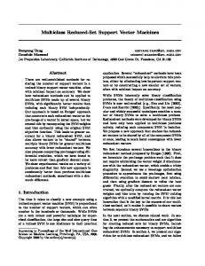
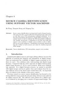
Marinos [3], the squeezing problems are divided into three classes associated with different levels of normalized convergence in this study, that is, nonsqueezing problems (with ε < 1%), minor squeezing problems (with 1% ≤ ε < 2.5%), and severe to extreme squeezing problems (with ε ≥ 2.5%), as shown in Figure 1 (Figure 1 is reproduced from Hoek and Marinos [3], under the Creative Commons Attribution License/Public Domain). The squeezing class labels are defined as 1 � nonsqueezing problems, 2 � minor squeezing problems, and 3 � severe to extreme squeezing problems. Figure 2 shows the histograms, cumulative distributions, and additional statistics, including the number of data (N), minimum and maximum values (Min and Max), means (Mean), and standard deviations (Std. Dev.) of D, H, Q, K, and ε. According to Figure 2(f), among the total 117 case histories, 33 cases are nonsqueezing tunnels with ε < 1%, 24 cases are minor squeezing tunnels with 1% ≤ ε < 2.5%, and the remaining 60 cases are severe to extreme squeezing tunnels with ε ≥ 2.5%. Note that only 56 case histories in our database reported specific values of K and the remaining provided information allowing us to compute the values of K using the methods described below [20]: (a) Stiffness of concrete or shotcrete linings Assuming that a closed ring of concrete or shotcrete is installed in a circular tunnel, its elastic stiffness, Kc, can be expressed as [23] 2

2. Database Description We compiled a database based on an extensive literature review, including a total of 117 datasets obtained from different countries, such as India, Nepal, Bhutan, Venezuela, China, Austria, and Greece. All the datasets contained the values of diameter (D), buried depth (H), support stiffness (K), rock tunneling quality index (Q), normalized convergence (%), and squeezing classes (1/2/3). Based on the five categories of squeezing problems in rock tunnels proposed by Hoek and

Kc �

Ec 􏽨R2 − R − tc 􏼁 􏽩

2 , 1 + vc 􏽨 1 − 2vc 􏼁R2 + R − tc 􏼁 􏽩

(1)

where Ec � elastic modulus of concrete or shotcrete, vc � Poisson’s ratio of concrete or shotcrete, R � radius of tunnel, and tc � thickness of concrete or shotcrete ring. (b) Stiffness of steel sets The effective stiffness of a steel set with backfill, Ksb, can be estimated as [16]

3 Strain, ε = tunnel closure/tunnel diameter∗100

Advances in Civil Engineering

15 14 13 12 11 10 9 8 7 6 5 4 3 2 1 0

δ

3

ε greater than 2.5% Severe to extreme squeezing problems

r0

ε between 1 and 2.5% Minor squeezing problems

ε less than 1% Nonsqueezing problems 1 0.2 0.3 0.4 0.5 0.6 σcm/po = rock mass strength/in situ stress 2

0.1

Figure 1: Multiclass squeezing problems with different levels of normalized convergence (modified from Hoek and Marinos [3]).

R Ksb � p , u where p � monitored radial support u � measured radial deformation.

(2) pressure

and

(c) Stiffness of ungrouted rock bolts and cables The stiffness of an ungrouted rock bolt or cable, Kb, can be computed as [23]: 1 ss 4l � c l􏼢 + Qld 􏼣, R πdb Eb Ksb

(3)

where sc � circumferential spacing of rock bolts or cables, sl � longitudinal spacing of rock blots or cables, l � free length of rock bolts or cables, db � diameter of rock bolts or cables, Eb � elastic modulus of rock bolts or cables, and Qld � a load-displacement constant (in units of displacement/force). (d) Stiffness of combined support systems Assuming that several support systems are installed together at the same time, their combined stiffness can be computed as the summation of their individual support stiffness [23].

3. Multiclass Support Vector Machine (SVM) Method 3.1. Classic SVM Method. The support vector machine (SVM) is a type of the machine learning method developed based on statistical learning theory (SLT) [24, 25] and is extensively used as one of the most robust binary classifiers [1]. SVMs do not require prior knowledge of a particular model form, possess a flexible nonlinear modeling capability, and have high generalization performance. Therefore, they have become popular in various fields, such as mechanical engineering [26], biomedical engineering [27, 28], information and communication engineering [29], and agriculture [30]. They have also been employed in geotechnical engineering [31–35].

In fact, the SVM is a classifier dividing the data into two groups by devising a hyperplane as a decision surface. In other words, the dataset is separated by the “optimal” hyperplane, as illustrated by the linearly separable case of Figure 3. Additionally, the reference used herein to “optimal” indicates that the distance between the nearest points to the hyperplane is maximized. As described below, the optimal decision plane could be determined by maximizing the margin of separation between the members of the two classes, that is, maximizing the classification margin between the decision boundary lines H1 and H2, which are parallel to the optimal classification line (or hyperplane). Assume that the dataset 􏼈(x1 , y1 ), . . . , (xN , yN )􏼉, y ∈ {−1, 1}, can be optimally separated by the hyperplane determined by the weight vector w and the bias b, that is, wTx + b � 0. The problem is equivalent to determining the parameters w and b which minimize the cost function [1]: 1 (4) f(w) � wT w, 2 subject to the constraints yi 􏼐wT x + b􏼑 ≥ 1 for i � 1, 2, . . . N.

(5)

For the maximal margin hyperplane, the solution to the above optimization problem is given by Vapnik [25] as follows: N

w � 􏽘 αi yi xi ,

(6)

i�1

1 b � − 􏼐wT xr + xs 􏼁􏼑, 2

(7)

where α represents the Lagrange multipliers and xr and xs are the support vectors satisfying the equations αr , αs > 0, yr � −1,

(8)

ys � 1. It is easy to prove that the Lagrange multipliers are positive real numbers that maximize

4

Advances in Civil Engineering N = 117 Min = 2.50 m Max = 13.00 m Mean = 6.40 m Std. dev. = 2.35 m

30 25

N = 117 Min = 52.00 m Max = 850.00 m Mean = 378.90 m Std. dev. = 207.21 m

100

25

80

20

80

15

60

10

40

20

5

20

0

0

100

40

(%)

15

Frequency

60 (%)

Frequency

20

10 5 0 2

3

4

5

6

0 50

7 8 9 10 11 12 13 D (m)

Frequency Cumulative %

190

330

470 610 H (m)

(a)

(b)

15

60

10

40

5

20

100 80

30

60 (%)

80 Frequency

20

N = 117 Min = 0.00 MPa Max = 5324.00 MPa Mean = 374.40 MPa Std. dev. = 711.30 MPa

40

100

(%)

Frequency

890


N = 117 Min = 0.00 Max = 93.50 Mean = 1.40 Std. dev. = 8.76

25

750

20 40 10

0

0

0 0

0.02

0.04

0.1 Q

0.5

5

20

100

0 0


20

40

100 1000 2000 5500 K (MPa)

Frequency Cumulative % (c)

(d)

N = 117 Min = 0.00% Max = 36.70% Mean = 3.90% Std. dev. = 5.47%

25

100

60

10

Frequency

60 (%)

Frequency

20

40

80

50

80

15

100

60

40

(%)

30

70

30

40

20 20

20

5

10 0

0 0

0 0

1

3

5 ε (%)

Frequency Cumulative % (e)

15

25

40

1

2 Squeezing classes

3


(f)

Figure 2: Histograms, cumulative distributions, and statistical evaluations of the experimental data.


5

Optimal hyperplane H

Sub-SVM23

{1,2,3}

H1 2

3 H2 {1,2}

Sub-SVM21 1

Sub-SVM13

2

3

{1,3}

1

Classification margin Class 2

Class 1 Class 2

Figure 3: Schematic diagram of optimal hyperplane. N i�1

1 N N 􏽘 􏽘 α α y y xT x , 2 i�1 j�1 i j i j i j

(9)

subject to N

􏽘 αi yi � 0,

αi > 0.

(10)

i�1

For nonlinear separable cases, the kernel function is often used to map the training data into a higher dimensional space where the data can be separated in an easier manner. The solutions for the kernel SVM could be similarly obtained by replacing the term xTi xj in (17) with K(xi , xj ). In addition, the corresponding hyperplane could be expressed as N

􏽘 αi K􏼐xi , xj 􏼑 + b � 0.

Class 3

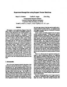
Figure 4: The structure of DAG-SVM used for three-class classification problems.

Support vector Support vector

􏽘 αi −

Class 1

(11)

i�1

The four basic kernel functions are as follows: (1) linear kernel function: K(xi , xj ) � xTi xj , (2) nth order polynomial kernel function: K(xi , xj ) � (xTi xj + 1)n , (3) radial basis function (RBF): K(xi , xj ) � exp(−(‖xi − xj ‖/2σ 2 )), and (4) sigmoid-kernel functions with parameters k and θ: K(xi , xj ) � tan h(k(xTi xj ) + θ). In this study, the most commonly used RBF kernel has been adopted because it has been reported that the RBF kernel could result in higher classification accuracy than the other kernels [22]. 3.2. Multiclass SVM. As previously discussed, the classical SVM classifiers were originally designed for binary classifications. However, there are more than two classes in some practical classification problems. For instance, one has to divide the potential squeezing effect into several classes according to the magnitude of the normalized convergence so that the severity of the squeezing could be adequately

assessed or predicted. This constitutes a typical multiclass classification problem. Two commonly used strategies for constructing multiclass SVM are the “one-against-one” and “one-againstall” approaches. In the “one-against-one” approach, we build one SVM for each pair of classes, which means that if there are k classes, then k(k − 1)/2 binary SVM classifiers are constructed to distinguish the samples of one class from the samples of another class. In the classification, we use a voting strategy, that is, each binary classification is considered to be a voting, whereby votes can be cast for all the samples. In the end, a point is designated to be part of a class with the maximum number of votes. However, in the one-against-all approach, we build as many binary classifiers as there are classes, and each trained classifier is used to separate one class from the rest. To predict a new instance, we choose the classifier with the largest decision function value. In this study, we used the directed acyclic graph SVM (DAG-SVM) approach that combines the SVM and the decision tree. The training process is the same as the “oneagainst-one” method, which also constructs k(k − 1)/2 binary SVM classifiers. However, the method uses a binary acyclic graph in the process of detection. If a binary decision tree is constructed for the k-class data samples, each leaf node of the tree corresponds to a class, and each nonleaf node corresponds to a sub-SVM classifier. Therefore, the decision tree has k(k − 1)/2 nonleaf nodes (i.e., the number of sub-SVM classifiers is k(k − 1)/2) and k leaf nodes (the number of classes is k). There are different schemes for constructing a strict DAG with k leaf nodes. For instance, the structure of a DAG-SVM for three-class classification problems is shown in Figure 4, where k indicates that x does not belong to class k. Starting at the root node (i.e., node “sub-SVM23”) for an input data sample x, we determine whether the left or right sub-SVM classifier (i.e., the nodes “sub-SVM21” or “sub-SVM13”) would be used depending on the output value. Subsequently, the class of the input data sample would be finally determined based on the output value of node “subSVM21” or “sub-SVM13”.

6


Table 2: Resultant accuracy and confusion matrices of 8-fold CV.

No. 1

93.33

6.67

No. 2

86.67

13.33

No. 3

80.00

20.00

No. 4

93.33

6.67

No. 5

80.00

20.00

No. 6

100.00

0.00

No. 7

80.00

20.00

No. 8

91.67

8.33

Average

88.13

11.87

Confusion matrices Actual 1 8 0 0 Actual 1 12 0 1 Actual 1 8 0 0 Actual 1 0 0 1 Actual 1 0 0 0 Actual 1 0 0 0 Actual 1 0 0 0 Actual 1 3 0 0

2 0 1 1

3 0 0 5

Predicted 1 2 3

2 0 0 1

3 0 0 1

Predicted 1 2 3

2 1 0 0

3 0 2 4

Predicted 1 2 3

2 3 Predicted 0 0 1 3 0 2 0 11 3 2 0 4 1

3 0 2 8

Predicted 1 2 3

2 3 Predicted 0 0 1 2 0 2 0 13 3 2 0 9 0

3 0 3 3

Predicted 1 2 3

2 0 0 1

3 0 0 8

Predicted 1 2 3

4. Results and Discussion 4.1. K-Fold Cross Validation. The aim of our proposed multiclass SVM classifier is to predict the severity of tunnel squeezing, and 8-fold cross validation is performed to estimate its validity in practice. Firstly, the original 117 datasets are equally divided into eight groups. Secondly, seven out of eight groups are used to train the multiclass SVM classifier with LibSVM [22], and the remaining group is left for validation purposes. Finally, the above process will be repeated eight times so that each case is predicted once in the entire database, and the cross validation accuracy is the percentage of data which are correctly classified. The corresponding classification accuracy and confusion matrices are listed in Table 2, and the average classification accuracy is

Class

Validation Accuracy Error rates groups (%) (%)

3

2

1 1

2

3

4

5

6 7 8 9 10 11 12 13 14 15 Cases for group No 1

Actual Predicted

Figure 5: Actual and predicted classification results of group No. 1.

approximately 88.1%. The confusion matrix could clearly show whether the class is misclassified (i.e., if a class is classified erroneously as another class) and describe the difference between the predicted and the actual classes. Furthermore, the sum of the elements on the principal diagonal represents the number of cases which are correctly classified. In addition, the sum of the elements off the principal diagonal represents the number of cases that are misclassified. When group No. 1 is used for model validation, the resultant classification results are shown in Figure 5. The horizontal axis represents the cases of the validation dataset (group No. 1). There are fifteen cases in total. The vertical axis represents the class of the cases. Only case No. 14 was misclassified as class 3 (i.e., ε > 2.5% with severe to extreme squeezing problems) since the actual class of case No. 14 is class 2 (i.e., 1% ≤ ε < 2.5% with minor squeezing problems), thereby indicating that the predicted result is conservative and safe. The classification accuracy is approximately 93.3%. 4.2. Comparison with Traditional Methods. In order to compare the performance of the proposed multiclass SVM classifier with that of the traditional methods, we have employed both the proposed multiclass SVM classifier and the empirical formula proposed by Singh [11] (i.e., H > 350Q1/3) to predict the squeezing class using all 117 datasets, and the results are listed in Table 3. Note that the accuracy for squeezing ground can be computed as the number of squeezing cases correctly classified divided by the total number of squeezing tunnels tested, the accuracy for nonsqueezing ground can be computed as the number of nonsqueezing cases correctly classified divided by the total number of nonsqueezing tunnels tested, and the overall accuracy can be computed as the number of tunnels correctly classified divided by total number of tunnels tested. From the total number of datasets, 94 cases were correctly classified using the empirical approach, and the


7

Table 3: Performance of the proposed approach, the empirical formula, and the two-class SVMs used to determine the squeezing. Method

Accuracy for squeezing ground (%) 82.1 79.4 86.9

Number of classes

Empirical formula Binary SVM Multiclass SVM

2 2 3

Accuracy for nonsqueezing ground (%) 78.8 88.1 93.9

Overall accuracy (%) 80.3 84.1 88.1

Table 4: Accuracy elicited using 8-fold CV with all parameters, without parameter K, and without parameter D. Accuracy with all four parameters (%) Accuracy without K (%) Accuracy without D (%)

No. 1 93.33 80.00 93.33

No. 2 86.67 60.00 86.67

No. 3 80.00 60.00 86.67

predicted accuracy was approximately 80.3% (i.e., 94/117). One probable reason for this relatively worse performance of the empirical formula proposed by Singh et al. [11] is that we have extended the original database employed in their work and constructed the multiclass SVM model based on the extended database. In addition, Shafiei et al. [1] used a more comprehensive database, including 198 tunnel cases, to construct their binary SVM classifier to predict the tunnel squeezing. Unfortunately, this comprehensive database cannot be directly used because their database contains only two input parameters, that is, H and Q, and does not provide any information about the other two parameters (i.e., K and D) considered in this study. The overall accuracy was reported to be equal to 84.1%, and the accuracy for squeezing ground was reported to be 79.4%. For multiclass SVM model, the overall accuracy and the accuracy for squeezing ground are 88.1% and 86.9% (Table 3), respectively, showing that the multiclass SVM model performs slightly better than the binary SVM classifier. As shown in Table 3, for the multiclass SVM model, the accuracy for nonsqueezing ground is higher than that for the squeezing ground, indicating a relatively “conservative” (and safe) model. Instead of predicting the class, many applications require posterior class probability which can be approximated by a sigmoid function (see Platt [36] for detailed descriptions) and such posterior probabilities can be used to assess the acceptability of the prediction [1]. For instance, let us imagine a new tunnel whose design is considered with K � 20 MPa, H � 200 m, Q � 0.4, and D � 6.0 m. The posterior probability P (y � 1|x) can be estimated as 78.3%, indicating that there is probably nonsqueezing problems for this tunnel, and this prediction is accepted with high confidence. And the posterior probability could be useful in tunnel risk analyses. In general, our approach performs slightly better than the empirical approach and the classical binary SVM in terms of the classification accuracy. Additionally, the empirical approach and the binary SVM classifier can only make a binary classification; that is, it can only predict whether squeezing occurs but cannot predict the severity of squeezing. Finally, it is important to mention that, as discussed by Jimenez and Recio [6, 37], the proposed multiclass SVM model should not be considered as a “final solution” and it should be expected to

No. 4 93.33 80.00 73.33

No. 5 80.00 73.33 86.67

No. 6 100.00 73.33 86.67

No. 7 80.00 73.33 66.67

No. 8 91.67 91.67 91.67

Average 88.13 73.96 83.96

be further updated and improved as more tunnel squeezing cases are included in the training database. 4.3. Influence of Support Stiffness and Tunnel Diameter. Tunnel deformation may be effectively controlled by installing appropriate support systems at a proper time. In other words, the squeezing condition could be influenced by the support stiffness applied to the tunnel. However, few studies have employed support stiffness as one of the input parameters to predict tunnel squeezing [16]. In order to assess the influence of support stiffness on tunnel squeezing, the support stiffness (K) is removed from the four input parameters (i.e., diameter (D), depth (H), support stiffness (K), and rock tunneling quality index (Q)); that is, the tunnel squeezing is predicted based on the remaining three parameters, that is, Q, H, and D. The 8-fold CV method is used again to validate the trained multiclass SVM using only three input parameters. The results are listed in Table 4. If the support stiffness is removed, the average accuracy obtained is reduced from 88.1% to 74.0%, showing that support stiffness has a significant influence on the classification accuracy of tunnel squeezing. Similarly, the influence of tunnel diameter can be assessed, and the results are also listed in Table 4. The resultant average accuracy is slightly reduced from 88.1% to 84.0%, indicating that tunnel diameter does not seem to have a significant influence on the predictive capabilities of the proposed model. This observation is coincident with the study by Jimenez and Recio [37]. In addition, we performed analysis of variance (ANOVA) to demonstrate the significance of these two parameters, namely, K and D, and the significance values for K and D are 0.046 and 0.004, respectively, indicating that the influence of K and D on tunnel squeezing is significant.

5. Conclusions A multiclass SVM classifier was developed to predict the tunnel squeezing based on four input parameters: diameter (D), depth (H), support stiffness (K), and rock tunneling quality index (Q). An “one-against-one” approach was employed to train the classifier from 117 available training datasets obtained from previous studies (Table 5). The 8-fold

8

Advances in Civil Engineering TABLE 5

No. D (m) H (m) Q K (MPa) ε (%) Class 1 6.0 150.0 0.400 26.19 0.42 1 2 6.0 200.0 0.400 20.00 0.75 1 3 5.8 350.0 0.500 2.53 7.90 3 4 4.8 225.0 3.600 1000.00 0.06 1 5 4.8 340.0 1.800 500.00 0.40 1 6 4.8 550.0 5.100 1600.00 0.05 1 7 12.0 220.0 0.800 32.89 0.38 1 8 13.0 52.0 15.000 16.67 0.18 1 9 3.0 280.0 0.050 9.80 2.80 3 5.96

4.50

3

Chibro-Khodri tunnel

India

0.050

9.90

6.00

3


India

0.022

48.56

2.00

2


India

100.0

0.005

88.96

2.62

3

Nepal

4.0

112.0

0.006

71.28

1.19

2

Nepal

Sericite schists

[41]

15 16

4.3 4.0

111.0 112.0

0.008 0.008

1936.00 936.00

0.75 0.20

1 1

Nepal Nepal

4.0

112.0

0.008

651.00

0.10

1

18 19 20

4.0 4.2 4.0

140.0 100.0 138.0

0.009 0.010 0.013

430.00 31.72 1934.00

0.80 3.81 0.19

1 3 1

21

4.4

212.0

0.040

5324.00

0.02

1

22

5.0

300.0

0.050

1430.00

0.18

1

Khimti 1 hydroproject A3 ch345

Nepal

23

4.0

112.0

0.060

458.00

0.30

1

Nepal

24

4.0

95.0

0.065

933.00

0.29

1

Nepal

Gneiss

[41]

25

4.0

218.0

0.070

739.00

0.14

1

Khimti 1 hydroproject A1 ch665 Khimti 1 hydroproject A2 ch1730 Khimti 1 hydroproject A4 ch550

Sheared schists Gneiss Clay-filled sheared gneiss Schists Sheared schists Sericite schists Gneiss and sericite schists Gneiss and sericite schists Gneiss and schists

[41] [41]

17

Khimti 1 hydroproject A1 ch515 Khimti 1 hydroproject A4 ch1013 Khimti 1 hydroproject A1 ch580 Khimti 1 hydroproject A4 ch974 Khimti 1 hydroproject A4 ch1045 Khimti 1 hydroproject A3 ch220 Khimti 1 hydroproject A1 ch500 Khimti 1 hydroproject A2 ch601 Khimti 1 hydroproject A2 ch1283

Rock type Clay conglomerate Clay conglomerate — Fractured quartzite Sheared metabasics Foliated metabasics Argillaceous phyllite Banded schists Crushed red shales Soft and plastic black clays Seamy crushed red Soft and plastic black clays Sheared schists

Nepal

[41]

26

4.0

98.0

0.080

933.00

0.77

1


Nepal

27

5.0

284.0

0.090

68.55

1.24

2


Nepal

28

5.0

300.0

0.090

664.29

0.28

1


Nepal Nepal

Chlorite sericite gneiss Gneiss and sericite schists Gneiss Gneiss and sericite schists Banded gneiss and chlorite schists Gneiss and chlorite schists Gneiss and sericite schists Gneiss and schists Gneiss and schists Gneiss and schists Gneiss and schists Gneiss Banded gneiss Banded gneiss — Fractured quartzite Laminated metabasics Sheared metabasics Sheared metabasics Metavolcanic Metavolcanic Metavolcanic Metavolcanic Crushed phyllites

10

3.0

280.0

0.022

11

9.0

680.0

12

9.0

280.0

13

4.2

14

Tunnel Khara hydroproject Khara hydroproject Maneri stage I Maneri-Bhali hydroproject Maneri-Uttarkashi power Maneri-Uttarkashi power Tehri dam project Upper Krishna project Chibro-Khodri tunnel

Location India India India India India India India India India

Nepal Nepal Nepal Nepal Nepal

29

4.0

261.0

0.095

931.00

0.15

1


30

4.0

198.0

0.140

934.00

0.29

1


Nepal

31

4.0

225.0

0.140

1430.00

0.24

1


Nepal

32 33 34 35 36 37 38 39 40 41 42 43 44 45 46 47 48

5.0 4.1 5.0 5.0 4.0 4.0 4.0 4.6 4.8 4.8 7.0 7.0 7.0 2.5 7.0 2.5 4.6

130.0 158.0 276.0 276.0 126.0 114.0 114.0 300.0 350.0 800.0 285.0 410.0 415.0 480.0 500.0 510.0 240.0

0.200 0.230 0.250 0.280 0.300 0.470 0.600 0.023 0.500 2.500 0.100 0.300 0.880 0.800 1.000 0.880 0.120

936.00 650.00 940.00 652.00 461.00 648.00 556.00 7.71 25.32 48.99 9.79 9.79 9.79 9.84 9.79 9.84 3.97

0.34 0.32 0.77 0.56 0.03 0.03 0.24 7.00 7.90 8.90 2.87 2.80 2.19 2.88 2.64 2.42 4.50

1 1 1 1 1 1 1 3 3 3 3 3 2 3 3 2 3

Khimti 1 hydroproject A3 ch15 Khimti 1 hydroproject A3 ch59 Khimti 1 hydroproject A3 ch200 Khimti 1 hydroproject A3 ch210 Khimti 1 hydroproject A2 ch441 Khimti 1 hydroproject A4 ch852 Khimti 1 hydroproject A4 ch876 Loktak hydro Maneri-Bhali stage I Maneri-Uttarkashi power Maneri stage II tunnel Maneri stage II tunnel Maneri stage II tunnel Maneri stage II tunnel Maneri stage II tunnel Maneri stage II tunnel Giri-Bata tunnel

Nepal Nepal Nepal Nepal Nepal Nepal Nepal India India India India India India India India India India

Reference [38, 39] [38, 39] [38] [39, 40] [40] [40] [38, 39] [38, 39] [15, 38] [38] [38] [38] [41]

[41] [41] [41] [41] [41] [41] [41]

[41] [41] [41] [41] [41] [41] [41] [41] [41] [41] [41] [41] [41] [38] [15, 40] [15, 40] [42, 43] [42, 43] [42, 43] [42, 43] [42, 43] [42, 43] [42–44]


9 Table 5: Continued.

No. D (m) H (m) 49 4.6 440.0 50 4.6 450.0 51 4.6 400.0 52 4.6 400.0 53 4.6 200.0 54 4.6 325.0 55 4.6 400.0 56 5.8 700.0 57 5.8 550.0 58 5.8 635.0 59 5.8 650.0 60 5.8 450.0 61 5.8 750.0 62 7.0 450.0

Q 0.050 0.060 0.030 0.050 0.020 0.030 0.512 0.300 1.700 4.000 4.120 0.310 0.500 0.590

K (MPa) 3.97 3.97 3.98 3.98 2.98 2.98 2.98 9.81 9.81 9.81 9.81 5.10 8.10 9.67

ε (%) Class 10.04 3 10.30 3 10.43 3 7.61 3 6.20 3 8.75 3 0.67 1 4.83 3 2.66 3 2.33 2 2.07 2 4.83 3 4.14 3 3.00 3

Location India India India India India India India India India India India India India India

3 3 2

Tunnel Giri-Bata tunnel Giri-Bata tunnel Giri-Bata tunnel Giri-Bata tunnel Giri-Bata tunnel Giri-Bata tunnel Giri-Bata tunnel Maneri stage I tunnel Maneri stage I tunnel Maneri stage I tunnel Maneri stage I tunnel Maneri stage I tunnel Maneri stage I tunnel Noonidih colliery Tala hydro-HRT, tala HRT, Bhutan Tala HRT, Bhutan Tala HRT, Bhutan Tala HRT, Bhutan

63

6.8

337.0

0.007

44.76

2.10

2

64 65 66

6.8 6.8 6.8

337.0 337.0 337.0

0.011 0.006 0.006

16.05 22.58 36.36

3.80 3.10 2.20

67

6.8

337.0

0.080

14.09

2.20

2

Tala HRT, Bhutan

Bhutan

68 69 70 71 72 73 74 75 76 77 78 79 80 81 82 83 84 85 86 87 88 89 90 91 92

8.7 8.7 8.7 8.7 8.7 8.7 8.7 8.7 8.7 8.7 8.7 8.7 8.7 8.7 8.7 8.7 11.0 11.0 11.0 11.0 11.0 11.0 11.0 11.0 11.0

550.0 600.0 600.0 600.0 600.0 620.0 620.0 620.0 620.0 620.0 620.0 620.0 580.0 580.0 550.0 575.0 700.0 700.0 750.0 600.0 850.0 600.0 300.0 400.0 800.0

0.029 0.023 0.030 0.018 0.023 0.020 0.008 0.009 0.009 0.016 0.020 0.025 0.023 0.025 0.025 0.007 0.417 0.333 0.333 0.250 0.056 0.033 0.001 0.003 0.194

39.13 90.71 34.48 26.20 28.48 26.20 14.67 14.67 14.67 26.20 26.10 50.80 26.20 74.66 39.87 21.17 7.43 9.14 9.14 9.14 20.40 33.33 16.50 17.00 17.14

2.30 1.40 2.90 3.90 3.20 4.90 8.50 7.70 8.20 4.40 4.10 2.50 3.70 1.70 2.40 6.00 3.50 3.50 3.50 3.50 5.00 3.00 6.00 6.00 3.50

2 2 3 3 3 3 3 3 3 3 3 3 3 2 2 3 3 3 3 3 3 3 3 3 3

Kaligandaki “A” HRT Kaligandaki “A” HRT Kaligandaki “A” HRT Kaligandaki “A” HRT Kaligandaki “A” HRT Kaligandaki “A” HRT Kaligandaki “A” HRT Kaligandaki “A” HRT Kaligandaki “A” HRT Kaligandaki “A” HRT Kaligandaki “A” HRT Kaligandaki “A” HRT Kaligandaki “A” HRT Kaligandaki “A” HRT Kaligandaki “A” HRT Kaligandaki “A” HRT Nathpa Jhakri-HRT Nathpa Jhakri-HRT Nathpa Jhakri-HRT Nathpa Jhakri-HRT Nathpa Jhakri-HRT Nathpa Jhakri-HRT Nathpa Jhakri-HRT Nathpa Jhakri-HRT Nathpa Jhakri-HRT

Nepal Nepal Nepal Nepal Nepal Nepal Nepal Nepal Nepal Nepal Nepal Nepal Nepal Nepal Nepal Nepal India India India India India India India India India

93

6.5

300.0

0.033

10.00

3.00

3

Udhampur rail tunnel (T1)

India

94

6.5

312.0

0.094

34.67

1.50

2


India

95

6.5

280.0

0.083

29.33

1.50

2


India

96

6.5

270.0

0.125

15.91

2.20

2


India

97

6.5

285.0

0.063

12.80

2.50

3


India

Bhutan Bhutan Bhutan Bhutan

Rock type Reference Crushed phyllites [42–44] Crushed phyllites [42–44] Crushed phyllites [42–44] Crushed phyllites [42–44] Crushed phyllites [42–44] Crushed phyllites [42–44] Crushed slates [42–44] Sheared metabasics [42, 45] Siliceous phyllites [42, 45] Foliated metabasics [42, 45] Siliceous phyllites [42, 45] Sheared metabasics [42, 45] Crushed quartzite [42, 45] Weak coal [45] AGO (adverse [46] geological [46] occurrences): [46] completely sheared, [46] highly weathered biotite schist associated with banded gneiss, amphibolites, and [46] quartzites in thin bands Graphitic phyllite [47, 48] Graphitic phyllite [47, 48] Graphitic phyllite [47, 48] Graphitic phyllite [47, 48] Graphitic phyllite [47, 48] Graphitic phyllite [47, 48] Graphitic phyllite [47, 48] Graphitic phyllite [47, 48] Graphitic phyllite [47, 48] Siliceous phyllites [47, 48] Graphitic phyllite [47, 48] Graphitic phyllite [47, 48] Graphitic phyllite [47, 48] Graphitic phyllite [47, 48] Graphitic phyllite [47, 48] Graphitic phyllite [47, 48] [49] [49] [49] Quartz mica schist, [49] schistose quartzites, [49] and amphibolites [49] [49] [49] [49] Claystone, silty [49] claystone Claystone, silty [49] claystone Claystone, silty [49] claystone Claystone, silty [49] claystone Claystone, silty [49] claystone

10

Advances in Civil Engineering Table 5: Continued.

No. D (m) H (m)

Q

K (MPa) ε (%) Class

98

6.5

280.0

0.031

11.54

2.60

3


India

99

6.5

280.0

0.042

12.50

2.40

2


India

100

6.0

727.0

2.287

5.88

1.70

2

Chenani–Nashri escape tunnel

India

101

6.0

736.0

2.426

7.69

1.30

2


India

102

6.0

733.0

2.903

6.25

1.60

2


India

103

6.0

690.0

1.650

9.38

1.60

2


India

104

13.0

577.0

1.517

11.11

1.80

2

India

105

5.4

199.7

0.020

1217.16

4.58

3

Nepal

Dolomite

[50]

106

5.4

217.5

0.013

1217.16

25.54

3

Nepal

Dolomite

[50]

107

5.4

252.2

0.010

1523.07

12.50

3

Nepal

Brownish

[50]

108

5.4

246.3

0.010

1523.07

3.80

3

Nepal

Foliated phyllite

[50]

109

5.4

283.9

0.008

1645.38

36.73

3

Nepal

Talcose phyllite

[50]

110

5.4

284.5

0.008

1828.98

30.19

3

Nepal

Talcose phyllite

[50]

111

5.4

210.8

0.010

1575.72

18.30

3

Nepal

Talcose phyllite

[50]

112

5.4

237.7

0.010

1575.72

10.96

3

Nepal

Talcose phyllite

[50]

113

5.4

230.0

0.015

1217.16

9.80

3

Nepal

Foliated phyllite

[50]

114

5.4

222.6

0.015

1217.16

1.20

2

Nepal

Foliated phyllite

[50]

115 116 117

5.4 5.4 5.4

80.0 190.0 130.0

93.500 7.450 1.530

0.00 0.00 0.00

0.00 0.00 0.00

1 1 1

Chenani–Nashri escape tunnel Chameliya hydroelectric project headrace tunnel 3 + 172 Chameliya hydroelectric project headrace tunnel 3 + 190 Chameliya hydroelectric project headrace tunnel 3 + 296 Chameliya hydroelectric project headrace tunnel 3 + 314 Chameliya hydroelectric project headrace tunnel 3 + 404 Chameliya hydroelectric project headrace tunnel 3 + 420 Chameliya hydroelectric project headrace tunnel 3 + 681 Chameliya hydroelectric project headrace tunnel 3 + 733 Chameliya hydroelectric project headrace tunnel 3 + 764 Chameliya hydroelectric project headrace tunnel 3 + 795 Austria (Oetscher unit) Austria (Oetscher unit) Austria (Oetscher unit)

Rock type Claystone, silty claystone Claystone, silty claystone Siltstone, silty claystone Siltstone, silty claystone Siltstone, silty claystone Siltstone, silty claystone Siltstone

Austria Austria Austria

— — —

[51] [51] [51]

cross validation method was used to validate the constructed multiclass SVM classifier, and the results showed that the average error percentage was approximately 11.87%, which is considered acceptable for practical engineering applications. The proposed multiclass SVM classifier elicited some improvements compared to the traditional empirical formula proposed by Singh et al. [11] and the binary SVM classifier proposed by Shafiei [1], as it yielded higher accuracy and allowed the prediction of the squeezing severity. The proposed multiclass SVM classifier can be used for the preliminary classification of tunnel squeezing. However, it is not a substitute for more sophisticated methods, such as numerical simulation, wherein many other factors can be considered, such as the time effect of rock masses. The proposed approach can be further updated and improved as additional tunnel squeezing cases become available for training.

Additional Points Data Availability. The detailed data, including 117 tunnel cases, associated with this article are listed in Table 5.

Tunnel

Location

Reference [49] [49] [49] [49] [49] [49] [49]

Conflicts of Interest The authors declare that they have no conflicts of interest.

Acknowledgments This work was supported by the Natural Science Foundation of Shandong Province (Grant no. ZR2016EEB11); the Qilu Transportation Development Group (Grant nos. 2016QL02070001 and 2016B20); and the University of Jinan (Grant no. XBS1648).

References [1] A. Shafiei, H. Parsaei, and M. Dusseault, “Rock squeezing prediction by a support vector machine classifier,” in Proceedings of 46th US Rock Mechanics/Geomechanics Symposium, Chicago, IL, USA, June 2012. [2] R. Ajalloeian, B. Moghaddam, and A. Azimian, “Prediction of rock mass squeezing of T4 tunnel in Iran,” Geotechnical & Geological Engineering, vol. 35, no. 2, pp. 747–763, 2017.

Advances in Civil Engineering [3] E. Hoek and P. Marinos, “Predicting tunnel squeezing problems in weak heterogeneous rock masses,” Tunnels and Tunnelling International, vol. 32, no. 11, pp. 45–51, 2000. [4] S. Sakurai, “Displacement measurements associated with the design on underground openings,” in Proceedings of International Symposium on Field Measurements in Geomechanics, Zurich, Switzerland, September 1983. [5] J. C. Chern, C. W. Yu, and H. C. Kao, “Tunneling in squeezing ground,” in Proceedings of Fourth International Conference on Case Histories in Geotechnical Engineering, St. Louis, MO, USA, March 1998. [6] R. Jimenez and D. Recio, “A linear classifier for probabilistic prediction of squeezing conditions in Himalayan tunnels,” Engineering Geology, vol. 121, no. 3-4, pp. 101–109, 2011. [7] N. Phienwej, P. Thakur, and E. Cording, “Time-dependent response of tunnels considering creep effect,” International Journal of Geomechanics, vol. 7, no. 4, pp. 296–306, 2007. [8] Z. Guan, Y. Jiang, Y. Tanabashi, and H. Huang, “A new rheological model and its application in mountain tunnelling,” Tunnelling and Underground Space Technology, vol. 23, no. 3, pp. 292–299, 2008. [9] D. Sterpi and G. Gioda, “Visco-plastic behaviour around advancing tunnels in squeezing rock,” Rock Mechanics and Rock Engineering, vol. 42, no. 2, pp. 319–339, 2009. [10] J. L. Jethwa, B. Singh, and B. Singh, “Estimation of ultimate rock pressure for tunnel linings under squeezing rock conditions-a new approach,” in Proceedings of ISRM Symposium on Design and Performance of Underground Excavations, Cambridge, UK, September 1984. [11] B. Singh, J. L. Jethwa, A. K. Dube, and B. Singh, “Correlation between observed support pressure and rock mass quality,” Tunnelling & Underground Space Technology, vol. 7, no. 1, pp. 59–74, 1992. ¨ Aydan, T. Akagi, and T. Kawamoto, “The squeezing potential [12] O. of rocks around tunnels; theory and prediction,” Rock Mechanics and Rock Engineering, vol. 26, no. 2, pp. 137–163, 1993. [13] G. Barla, “Squeezing rocks in tunnels,” ISRM News Journal, vol. 2, no. 3-4, pp. 44–49, 1995. [14] R. Bhasin and E. Grimstad, “The use of stress-strength relationships in the assessment of tunnel stability,” Tunnelling and Underground Space Technology, vol. 11, no. 1, pp. 93–98, 1996. [15] E. Hoek, “Big tunnels in bad rock,” Journal of Geotechnical and Geoenvironmental Engineering, vol. 127, no. 9, pp. 726– 740, 2001. [16] R. D. Dwivedi, M. Singh, M. N. Viladkar, and R. K. Goel, “Prediction of tunnel deformation in squeezing grounds,” Engineering Geology, vol. 161, pp. 55–64, 2013. [17] J. Yao, B. Yao, L. Li, and Y. Jiang, “Hybrid model for displacement prediction of tunnel surrounding rock,” Neural Network World, vol. 22, no. 3, p. 263, 2012. [18] S.-j. Li, H.-b. Zhao, and Z.-l. Ru, “Deformation prediction of tunnel surrounding rock mass using CPSO-SVM model,” Journal of Central South University, vol. 19, no. 11, pp. 3311–3319, 2012. [19] S. Mahdevari and S. R. Torabi, “Prediction of tunnel convergence using artificial neural networks,” Tunnelling and Underground Space Technology, vol. 28, pp. 218–228, 2012. [20] X. Feng and R. Jimenez, “Predicting tunnel squeezing with incomplete data using Bayesian networks,” Engineering Geology, vol. 195, pp. 214–224, 2015. [21] Y. Alimohammadlou, A. Najafi, and C. Gokceoglu, “Estimation of rainfall-induced landslides using ANN and fuzzy clustering methods: a case study in Saeen Slope, Azerbaijan Province, Iran,” CATENA, vol. 120, pp. 149–162, 2014.

11 [22] C. C. Chang and C. J. Lin, “LibSVM: a library for support vector machines,” ACM Transactions on Intelligent Systems & Technology, vol. 2, no. 3, pp. 1–27, 2011. [23] E. Hoek and E. T. Brown, Underground Excavations in Rock, Institution of Mining and Metallurgy, London, UK, 1980. [24] C. J. C. Burges, “A tutorial on support vector machines for pattern recognition,” Data Mining & Knowledge Discovery, vol. 2, no. 2, pp. 121–167, 1998. [25] V. Vapnik, The Nature of Statistical Learning Theory, Springer-Verlag, New York, NY, USA, 1995. [26] H. N. Nguyen and H. H. Lee, “An enhanced SVM method to drive matrix converters for zero common-mode voltage,” IEEE Transactions on Power Electronics, vol. 30, no. 4, pp. 1788–1792, 2015. [27] P. N. Kumar and H. Kareemullah, “EEG signal with feature extraction using SVM and ICA classifiers,” in Proceedings of the International Conference on Information Communication and Embedded Systems, Chennai, India, February 2015. [28] B. H. Brinkmann, E. E. Patterson, C. Vite et al., “Forecasting seizures using intracranial EEG measures and SVM in naturally occurring canine epilepsy,” PLoS One, vol. 10, no. 8, article e0133900, 2015. [29] W. H. Lin and A. Hauptmann, “News video classification using svm-based multimodal classifiers and combination strategies,” in Proceedings of the Tenth ACM International Conference on Multimedia, Juan les Pins, France, December 2002. [30] K. Zolfaghari, J. Shang, H. Mcnairn, J. Li, and S. Homyouni, “Using support vector machine (SVM) for agriculture land use mapping with SAR data: preliminary results from western Canada,” in Proceedings of the International Conference on Agro-Geoinformatics, Fairfax, VA, USA, August 2013. [31] C. Youkuo and Y. Yongguo, “Forecasting of mine discharge based on phase space reconstruction and LS-SVM within the Bayesian evidence framework,” Electronic Journal of Geotechnical Engineering, vol. 20, no. 2, pp. 435–448, 2015. [32] C. Zhou and K. Yin, “Landslide displacement prediction of WA-SVM coupling model based on chaotic sequence,” Electronic Journal of Geotechnical Engineering, vol. 19, pp. 2973–2987, 2014. [33] F. Xu, B. Q. Huang, and K. Wang, “Study and application of slope displacement back analysis based on SVM-CTS,” Applied Mechanics & Materials, vol. 353–356, pp. 163–166, 2013. [34] W. Qin and H. Huang, “Parameters value selection of SVM for landslide displacement prediction,” Electronic Journal of Geotechnical Engineering, vol. 18, pp. 5185–5191, 2013. [35] A. T. C. Goh and S. H. Goh, “Support vector machines: their use in geotechnical engineering as illustrated using seismic liquefaction data,” Computers & Geotechnics, vol. 34, no. 5, pp. 410–421, 2007. [36] J. C. PIatt, “Probabilistic outputs for support vector machines and comparisons to regularized likelihood methods,” in Advances in Large Margin Classiers, MIT Press, Cambridge, MA, USA, 1999. [37] R. Jiménez and D. Recio, “Probabilistic prediction of squeezing in tunneling under high-stress conditions,” in Proceedings of the 12th ISRM Congress, Beijing, China, January 2012. [38] R. K. Goel, J. L. Jethwa, and A. G. Paithankar, “Indian experiences with Q and RMR systems,” Tunnelling and Underground Space Technology, vol. 10, no. 1, pp. 97–109, 1995. [39] M. Singh, B. Singh, and J. Choudhari, “Critical strain and squeezing of rock mass in tunnels,” Tunnelling and Underground Space Technology, vol. 22, no. 3, pp. 343–350, 2007. [40] R. K. Goel, J. L. Jethwa, and A. G. Paithankar, “Tunnelling through the young himalayas—a case history of the Maneri-

12

[41]

[42] [43] [44]

[45] [46]

[47]

[48]

[49] [50]

[51]

Advances in Civil Engineering Uttarkashi power tunnel,” Engineering Geology, vol. 39, no. 12, pp. 31–44, 1995. G. L. Shrestha, Stress Induced Problems in Himalayan Tunnels with Special Reference to Squeezing, Department of Geology and Mineral Resources Engineering, Norwegian University of Science and Technology, Trondheim, Norway, 2005. R. Goel, “Correlations for predicting support pressures and closures in tunnels,” Ph.D. thesis, Nagpur University, Nagpur, India, 1994. J. Choudhari, “Closure of underground opening in jointed rocks,” Ph.D. thesis, 2007. A. K. Dube, Geomechanical Evaluation of Tunnel Stability under Failing Rock Conditions in a Himalayan Tunnel, Department of Civil Engineering, University of Roorkee, Roorkee, India, 1979. J. L. Jethwa, Evaluation of Rock Pressures in Tunnels through Squeezing Ground in Lower Himalayas, University of Roorkee, Roorkee, India, 1981. S. Sripad, G. Raju, R. Singh, and R. Khazanchi, “Instrumentation of underground excavations at Tala Hydroelectric project in Bhutan,” in Proceedings of International Workshop on Experiences and Construction of Tala Hydroelectric Project Bhutan, New Delhi, India, June 2007. NEA, Geology and Geotechnical Report, Volume IV-A and Geological Drawings and Exhibits, Volume V-C, in Project Completion Report, N. E. Authority, Kaligandaki “A” Hydroelectric Project, Syanga, Nepal, 2002. K. K. Panthi and B. Nilsen, “Uncertainty analysis of tunnel squeezing for two tunnel cases from Nepal Himalaya,” International Journal of Rock Mechanics and Mining Sciences, vol. 44, no. 1, pp. 67–76, 2007. N. Kumar, Rock Mass Characterisation and Evaluation of Supports for Tunnels in Himalaya, Department of Civil Engineering, Indian Institute of Technology Roorkee, Roorkee, India, 2002. C. B. Basnet, Evaluation on the Squeezing Phenomenon at the Headrace Tunnel of Chameliya Hydroelectric Project, Nepal, Department of Geology and Mineral Resources Engineering, Norwegian University of Science and Technology, Trondheim, Norway, 2013. R. Schwingenschloegl and C. Lehmann, “Swelling rock behaviour in a tunnel: NATM-support vs. Q-support—a comparison,” Tunnelling and Underground Space Technology, vol. 24, no. 3, pp. 356–362, 2009.

International Journal of

Advances in

Rotating Machinery

Engineering Journal of

Hindawi www.hindawi.com

Volume 2018

The Scientific World Journal Hindawi Publishing Corporation http://www.hindawi.com www.hindawi.com

Volume 2018 2013

Multimedia

Journal of

Sensors Hindawi www.hindawi.com

Volume 2018


Volume 2018


Volume 2018

Journal of

Control Science and Engineering

Advances in

Civil Engineering Hindawi www.hindawi.com


Volume 2018

Volume 2018

Submit your manuscripts at www.hindawi.com Journal of

Journal of

Electrical and Computer Engineering

Robotics Hindawi www.hindawi.com


Volume 2018

Volume 2018

VLSI Design Advances in OptoElectronics International Journal of

Navigation and Observation Hindawi www.hindawi.com

Volume 2018



Chemical Engineering Hindawi www.hindawi.com

Volume 2018

Volume 2018

Active and Passive Electronic Components

Antennas and Propagation Hindawi www.hindawi.com

Aerospace Engineering


Volume 2018


Volume 2018

Volume 2018




Modelling & Simulation in Engineering

Volume 2018


Volume 2018

Shock and Vibration Hindawi www.hindawi.com

Volume 2018

Advances in

Acoustics and Vibration Hindawi www.hindawi.com

Volume 2018