are, in e ect, hallucinated. We also .... 1992 , and Bayesian algorithms Schultz and Stevenson, 1994 , is contained in the excellent paper by .... job of estimating the registration translation , the super-resolution results again omitted for brevity ...
Hallucinating Faces Simon Baker and Takeo Kanade CMU-RI-TR-99-32 Abstract In most surveillance scenarios there is a large distance between the camera and the objects of interest in the scene. Surveillance cameras are also usually set up with wide elds of view in order to image as much of the scene as possible. The end result is that the objects in the scene normally appear very small in surveillance imagery. It is generally possible to detect and track the objects in the scene, however, for tasks such as automatic face recognition and license plate reading, resolution enhancement techniques are often needed. Although numerous resolution enhancement algorithms have been proposed in the literature, most of them are limited by the fact that they make weak, if any, assumptions about the scene. We propose an algorithm that can be used to learn a prior on the spatial distribution of the image gradient for frontal images of faces. We proceed to show how such a prior can be incorporated into a super-resolution algorithm to yield 4-8 fold improvements in resolution (16-64 times as many pixels) using as few as 2-3 images. The additional pixels are, in e�ect, hallucinated. We also apply our algorithms to text data.
Keywords: Resolution enhancement, interpolation, super-resolution, learning, faces, text.
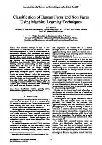
1 Introduction There is a large distance between the camera and the scene in most surveillance scenarios. Surveillance cameras are also usually set up with wide elds of view, in order to image as much of the world as possible. The end result is that objects of interest typically appear very small in surveillance imagery. Hence, for tasks such as automatic face and license plate recognition, resolution enhancement is usually needed. We are primarily interested in human faces in this paper. To gauge how di�cult resolution enhancement is for faces, we took a high resolution image of a face and repeatedly down-sampled it until it was unrecognizable. The results are shown in Table 1. The size of the initial image was 96 � 128 pixels, and at each step the image was down-sampled by a factor of 2 in each direction by averaging the pixel intensities. After 4 iterations, the image is 6 � 8 pixels and is no longer obviously an image of a face. The image begins to look like a face at around 12 � 16 pixels. For comparison, most face detectors use a window size of about 20 � 20 pixels [Rowley et al., 1998] [Sung and Poggio, 1999] [Schneiderman and Kanade, 1998]. Although these detectors res-ample the image to detect faces at di�erent scales, the 12 � 16 pixel image in Table 1 is approximately the smallest size at which they operate reliably. Determining the identity of the person in the 12 � 16 image, however, would be very di�cult, even for a human. It is only at approximately 24 � 32 pixels that identity begins to be recognizable. Most papers on face recognition do not give the size of the input images used, but typically the resolution is at least 96 � 128 pixels. For example, the faces in the FERET test set [Philips et al., 1997] are all at least this large. From Table 1, however, it appears that it should be possible to recognize faces at image sizes 48 � 64 pixels and above. Finally, facial features, such as the corners of the eyes and the mouth, are often used by facial analysis algorithms, for example, to determine where the person is looking [Gee and Cipolla, 1994] [Horsprasert et al., 1996]. 1
Table 1: A relatively high resolution (96 � 128 pixels) image of a face repeated down-sampled by pixel averaging. At around 24 � 32 pixels the facial features such as the corners of the eyes and the mouth are barely discernible, at around 12 � 16 pixels the identity of the person is very hard to recognize, and at around 6 � 8 pixels the image is not even clearly an image of a face.
96 � 128
48 � 64
24 � 32
12 � 16
6�8
Detect?
Yes
Yes
Yes
Maybe
No
Recognize?
Yes
Yes
Maybe
No
No
Features?
Yes
Maybe
No
No
No
These features are barely visible in the 48 � 64 pixel image, but in the 96 � 128 pixel image they can be seen clearly and localized accurately. Most automated face processing tasks should therefore be possible with (low noise) 96 � 128 pixel images. On the other hand, the smallest faces that can be reliably detected are approximately 12 � 16 pixels. In this paper, we will attempt to bridge this gap. We will develop a resolution enhancement algorithm, speci cally for faces, that can convert a small number (� 3) of 24 � 32 or 12 � 16 pixel images of a face into a single 96 � 128 pixel image.
1.1 Related Work: Single Image Interpolation One way of increasing the resolution of an image is to interpolate the pixel intensities. A wide variety of interpolation algorithms have been proposed, the most well known and frequently used being nearest-neighbor, bilinear, and variants of cubic spline interpolation [Pratt, 1991] [Wolberg, 1992]. A brief survey of several more sophisticated algorithms, including re ne2
Table 2: The RMS interpolation error (per pixel in grey levels) obtained using the standard
cubic B-spline algorithm [Wolberg, 1992] on a set of 596 faces like the one in Table 1. Each row corresponds to a xed input image size and each column to a xed output image size. These results show that, at least for faces, interpolation gets more di�cult as the images get smaller. in n out 12 � 16 24 � 32 48 � 64 96 � 128 48 � 64
11.9
24 � 32 12 � 16 6�8
26.1
15.5
22.2
20.4
29.2
33.9
36.7
42.4
45.4
ments to the cubic spline algorithms [Chen and deFigueiredo, 1985], regularization-based approaches [Karayiannis and Venetsanopolous, 1991], edge-preserving techniques [Xue et al., 1992], and Bayesian algorithms [Schultz and Stevenson, 1994], is contained in the excellent paper by Schultz and Stevenson [1996]. Another approach to interpolation is to learn how to interpolate from a set of high resolution training samples, together with corresponding low resolution versions of them. In [Freeman and Pasztor, 1999], the high resolution image is modeled as a Markov network, where each pixel is attached to its neighbors and the corresponding pixel in the low resolution image. Another approach suggested by John Platt [1999], might be to estimate the average cross-correlation (spectrum) of the high resolution training samples, and then use that as the input to the optimal linear interpolation algorithm proposed by Malvar and Staelin [1988]. While interpolation can give good results when the input images are fairly high resolution, it often performs worse as the input images get smaller, as is illustrated in Table 2. We took a set of 596 faces similar to the one in Table 1 and down-sampled them in the same manner. We then used the standard cubic B-spline algorithm [Wolberg, 1992] to reconstruct the higher resolution images. The RMS error per pixel over the entire set is presented in 3
Table 2 for various input/output size combinations. (The interpolation results for one of the 596 faces are shown in Figure 1.) The results show that, at least for faces, interpolation becomes much more di�cult as the image size gets smaller. Interpolating from 6 � 8 pixels to 12 � 16 pixels yields an RMS error of 26.1 grey-levels compared with only 11.9 interpolating from 48 � 64 to 96 � 128 pixels. The magni cation factor is the same in both cases, yet the results are far worse for the lower resolution image. If we wish to use 12 � 16 pixel images, we will therefore need to use more powerful techniques than single image interpolation.
1.2 Related Work: Multiple Image Super-Resolution It is possible to do much better if multiple images are available. It helps if there is some (small) relative motion between the camera and the scene, but motionless multiple image super-resolution is possible too [Elad and Feuer, 1997]. If there is relative motion, the rst step to super-resolution is to register the images; i.e. compute the motion of pixels from one image to the others. The motion is often assumed to take a simple parametric form [Bergen et al., 1992], but instead could be a full optical ow eld [Elad, 1996]. Once the pixel-wise correspondences between the images have been estimated, the low resolution input images need to be fused to form the high resolution image. A number of di�erent techniques have been proposed to do this, including, frequency domain approaches [Huang and Tsai, 1984] [Kim et al., 1990] [Ur and Gross, 1992] and edge-based approaches [Chiang and Boult, 1997]. Most approaches are, however, based on the constraints that the high resolution image, when appropriately warped and down-sampled, should yield the low resolution (input) images [Irani and Peleg, 1991] [Irani and Peleg, 1993]. These constraints can easily be embedded in a Bayesian framework with priors placed on the high resolution image [Schultz and Stevenson, 1996] [Hardie et al., 1997], and can be estimated recursively using a Kalman lter [Dellaert et al., 1998]. Several re nements and extensions have been 4
input n correct
12 � 16
24 � 32
48 � 64
48 � 64
�2
24 � 32
12 � 16
6�8
96 � 128
�2
�2
�4
�2
�4
�8
�4
�8
�16
Figure 1: The results for one of the images used in Table 2. As the resolution gets lower (i.e. moving down the rows), the interpolation results get worse, even for a xed magni cation of say �2 or �4. 5
proposed to the various super-resolution algorithms, including simultaneously computing structure [Cheeseman et al., 1994] [Shekarforoush et al., 1996], compensating for motion blur [Bascle et al., 1996], and dealing with varying illumination [Chiang and Boult, 1997]. For comparison, we implemented the algorithms of Schultz and Stevenson [1996] and Hardie et al. [1997] The results obtained using the Schultz and Stevenson algorithm on the same data as that used in Figure 1 are presented in Figure 2. The only slight di�erence is that the high resolution 96 � 128 pixel image was randomly translated multiple times before it was down-sampled to give the multiple inputs needed at lower resolutions. (We used enough input images so that the total number of pixels in all the low resolution images equals the number of pixels in the high resolution image. The results are similar even if either twice as many or half as many images are used, but are omitted for brevity.) On comparing Figures 1 and 2 we see that the super-resolution algorithm does perform signi cantly better than pure interpolation. The results for the 6 � 8 and 12 � 16 pixel images are still, however, far from perfect, even though enough images have been used that in the ideal case the high resolution image should be reconstructible. There are two possible reasons the performance is so poor. First, the registration (which is computed using the low resolution images) must be accurate relative to the size of the pixels in the high resolution image. When the ratio of the sizes of these pixels is 8{16, and the images are severely aliased, this task is very di�cult. We did, however, experiment with variants of the iterative registration algorithm in [Hardie et al., 1997] and found that, although it does do a very good job of estimating the registration (translation), the super-resolution results (again omitted for brevity) are not signi cantly improved by this step. We therefore suspect that the major cause of the poor performance is the second possibility, the grey level intensity noise. When the resolution is enhanced by a factor of 16 in each direction, any pixel in the high resolution image can be perturbed by 256 grey 6
input n correct
12 � 16
24 � 32
48 � 64
48 � 64
�2 (4 images)
24 � 32
12 � 16
6�8
96 � 128
�2 (4 images)
�4 (16 images)
�2 (4 images) �4 (16 images)
�8 (64 images)
�2 (4 images) �4 (16 images) �8 (64 images) �16 (256 images)
Figure 2: The results obtained using the super-resolution algorithm of Schultz and Stevenson [1996] on the data of Figure 1. The super-resolution algorithm does do much better than cubic B-spline interpolation, but the results for the larger magni cations are still poor. (See text for explanation.)
7
levels and still only change a handful of the pixels in the predicted low resolution images by just 1 grey level. Since we are working with 8-bit images, any algorithm that takes into account any noise in the input image intensities can therefore only impose fairly weak constraints on the high resolution images. The result is that the prior on the high resolution image becomes more important as the factor by which the resolution is enhanced gets larger. Since the Schultz and Stevenson prior [1996] is that the image has zero gradient, the results enhancing the resolution by 8{16 times contain much less high-frequency detail than they should. Removing the prior will, of course, not help. It will simply amplify the noise that is always present (even if only in the form of the discretization to an 8-bit intensity value.)
1.3 Class-Based Super-Resolution Using Gradient Priors The prior on the high resolution image therefore becomes relatively more important for larger magni cation factors. The Markov Random Field priors used by Schultz and Stevenson and Hardie at al. are too general to compensate for the fact that the image constraints are much weaker. In this paper, we propose an algorithm for learning a prior on the image gradient and show how it can be incorporated into a super-resolution algorithm. The speci c learning algorithm we use is based on the multi-resolution algorithm proposed by De Bonet and Viola for texture recognition [De Bonet and Viola, 1998], image de-noising [De Bonet and Viola, 1997], and random texture synthesis [De Bonet, 1997]. The super-resolution algorithm is a modi cation of the Schultz and Stevenson [1996] algorithm. Besides the choice of the learning algorithm, and the applicability of our algorithm to multiple images, the other major di�erence between our approach and the interpolation learning algorithm of Freeman and Pazstor [1999] is that our approach is \class-based" in the sense of [Riklin-Raviv and Shashua, 1999]. As will be shown, our results are a great improvement over previous methods, partly because they use multiple images, but partly 8
because the algorithms are dedicated to frontal images of faces. (We will also demonstrate that our approach works for text data when provided with an appropriate training set.) Another class-based approach is the recent work of Edwards et al. [1998]. In this paper, a parameterized model of a face, referred to as an active appearance model, is used to enhance the resolution of a video sequence. The parameters of the face model are estimated from the low resolution sequence, and then used to re-render a higher resolution version. Although closely related to our approach, it is unlikely that such an algorithm would work on images as small as 12 � 16 pixels. Active appearance models are based on the location of around 50 points on the face. When the image itself only contains 100-200 pixels, the triangulated elements on the model essentially become degenerate points.
2 Theory and Algorithms 2.1 Background: Gaussian, Laplacian, and Feature Pyramids We follow the non-parametric, multi-resolution approach of De Bonet and Viola [1997]. In this approach the images are decomposed as three types of pyramids; Gaussian pyramids, Laplacian pyramids, and feature pyramids. These pyramids are all illustrated in Figure 3. The Gaussian pyramid [Burt, 1980] [Burt and Adelson, 1983] of an image I , starting at level l = k, is the set of images Gk (I ); Gk (I ); : : :; GN (I ), where: 8 > (1) : REDUCE(Gl, (I )) if k < l � N +1
1
and N is chosen so that GN (I ) is (smaller than) some xed size. The operator REDUCE(�) combines a (Gaussian) smoothing step and a down-sampling step. The details of this operator vary somewhat from author to author. In [De Bonet, 1997], REDUCE(I ) = 2 # [I g], 9
G4
G4
G3
G3
G2
G2
G1 G0
(a) High Resolution Gaussian Pyramid
(b) Low Resolution Gaussian Pyramid
L4
H4
L3
H3
L2
(c) Laplacian Pyramid
V3
H2
L1 L0
V4
V2
H1 H0
V1 V0
(d) Feature (Derivative) Pyramids
Figure 3: (a) A Gaussian pyramid is created by repeatedly smoothing and down-sampling an image.
(b) Given a lower resolution image, we can create the pyramid starting at a higher level. Resolution enhancement can then be thought of as estimating the missing lower levels in the pyramid. (c) Each level of the Laplacian pyramid is de ned as the di�erence between the corresponding level of the Gaussian pyramid and the two-fold up-sampling (expansion) of the next higher level. The lowest level of the Gaussian pyramid G0 can be estimated from a higher level G2 by sub-sampling and adding the (appropriately sub-sampled) lower Laplacian levels L0 and L1 ; i.e. resolution enhancement can be performed by predicting the lower levels of the Laplacian pyramid. (d) Feature pyramids can also be generated from the Gaussian pyramid by taking horizontal and vertical derivatives. It is possible to use more sophisticated features, such as Freeman and Adelson's steerable lters [Freeman and Adelson, 1991].
10
where 2 # [�] is the two-fold down-sampling operator, and I g is the convolution of I with g, a two dimensional Gaussian kernel. We found the performance of our algorithms to be largely independent of the choice of the operator REDUCE(�). We actually chose REDUCE(�) to be the pixel averaging function: XX REDUCE(I )(m; n) = 14 I (2 � m + i; 2 � n + j ) (2) i j because the results using this de nition were slightly better, and also because this de nition is more consistent with image formation as integration over the pixel. The \Gaussian" pyramid of the 96 � 128 pixel image considered in Table 1 is illustrated in Figure 3(a). 1
1
=0 =0
In terms of the Gaussian pyramid, a resolution enhancement algorithm is a function from Gl(I ) to G (I ) where l > 0. Given a lower resolution image we can create a Gaussian pyramid starting at a higher level. For example, if the image is 2k times smaller (in each direction), we start at level l = k, as is illustrated in Figure 3(b) for k = 2. Resolution enhancement then consists of determining the missing lower levels Gk, (I ); : : : ; G (I ). 0
1
0
Like the Gaussian pyramid, the Laplacian pyramid [Burt and Adelson, 1983] consists of a set of images Lk (I ); Lk (I ); : : :; LN (I ). It is de ned in terms of the Gaussian pyramid as: 8 > < G (I ) , EXPAND(Gl (I )) if k � l < N Ll (I ) = > l (3) : Gl(I )) if l = N . where EXPAND(�) is the pixel replication (sub-sampling) operator: �m� �n� EXPAND(I )(m; n) = I ( 2 ; 2 ): (4) The Laplacian pyramid is useful for resolution enhancement because: +1
+1
G (I ) = EXPANDk (Gk (I )) + EXPANDk, (Lk, (I )) + : : : + EXPAND(L (I )) + L (I ): (5) 1
0
1
1
0
To estimate the high resolution image G (I ), the low resolution image Gk (I ) can be expanded the appropriated number of times, and the lower Laplacian levels (appropriately expanded) 0
11
added to it. To estimate G from G in Figure 3(b), we therefore just need to predict the Laplacian pyramid at the lower levels L and L . Figure 3(c) contains the Laplacian pyramid corresponding to the Gaussian pyramid in Figure 3(a). (The grey level of 127 corresponds to a Laplacian value of 0 for all of the levels except the top one L = G .) The lower levels of the Laplacian pyramid can be thought of as containing the high frequency components that must be added to the low resolution image to give the high resolution version. 0
2
0
1
4
4
The nal type of pyramid considered by De Bonet and Viola is a pyramid of \local texture measures" (or features) created using a lter bank. In [De Bonet, 1997], the lters are rst and second derivatives, but in later work steerable lters [Freeman and Adelson, 1991] are used. We used horizontal and vertical, rst and second derivative operators. The horizontal derivative pyramid is also a set of images Hk (I ); H (I ); : : :; HN (I ) de ned by: 1
Hl(I ) = Gl(I ) h for k � l � N
(6)
where h is a horizontal derivative kernel. The vertical derivative pyramid Vl(I ) and the second derivative pyramids Hl (I ) and Vl (I ) are de ned similarly. (We used (,1; 8; 0; ,8; 1)=16:0 for the rst derivative and (,1; ,2; 6; ,2; ,1)=12:0 for the second derivative.) The horizontal and vertical rst derivative pyramids of the Gaussian pyramid in Figure 3(a) are displayed in Figure 3(d). We did try di�erent de nitions of the features, but found the performance of our algorithms to be largely independent of the choice. 2
2
2.2 Predicting Laplacians and Gradient Priors We developed a modi cation of De Bonet's random sampling algorithm [De Bonet, 1997] to predict the lower levels of the Laplacian for resolution enhancement. Our algorithm is deterministic. It chooses the most likely values for the Laplacian (and the features) rather than randomly sampling from a set of likely values. For this reason, it is possible to perform the algorithm in one step from the low resolution image to the high resolution image. 12
Another di�erence is that (for faces) the decision is spatially variant. At each pixel, the algorithm only looks at the corresponding pixels in the training samples. It is able to do this: (1) because we have multiple training samples (unlike De Bonet who deliberately just uses a single texture example), and (2) because we take the class-based approach of [RiklinRaviv and Shashua, 1999] we know that the images are aligned. Hence, corresponding pixels are images of roughly the same point on the face. (For text data, De Bonet's assumption that the texture is spatially invariant is more appropriate and so we do use it. For text data, we use all of the pixels in all of the training samples to predict the Laplacian.) We describe our algorithm in terms of (a minor modi cation of) the \parent structure" vector introduced by De Bonet and Viola. Given an image I , its Laplacian and feature pyramids are constructed starting at some level. The l level parent structure at pixel (m; n) of image G (I ) is then the 5 � (N + 1 , l) dimensional vector: j k j k j k Sl(I )(m; n) = ( Ll (I )( ml ; nl ); Ll (I )( ml+1 ; ln+1 ); : : :; LN (I )( mN ; mN ) j k j k j k Hl(I )( ml ; nl ); Hl (I )( lm+1 ; ln+1 ); : : :; HN (I )( mN ; mN ) j k j k j k Vl (I )( ml ; nl ); Vl (I )( lm+1 ; ln+1 ); : : :; VN (I )( mN ; mN ) j k j k j k Hl (I )( ml ; nl ); Hl (I )( ml+1 ; ln+1 ); : : :; HN (I )( mN ; mN ) j k j k j k (7) Vl (I )( ml ; nl ); Vl (I )( lm+1 ; ln+1 ); : : : ; VN (I )( mN ; mN ) ): j k If (m; n) is a pixel in the i level of a pyramid, its parent at the i + 1 level is ( m ; n ). The parent structure therefore gets its name from the fact that it consists of the Laplacian and feature values of the l parent of (m; n), that pixel's parent, it's parent, and so on up to the top of the pyramids. See Figure 8 in [De Bonet, 1997] for an illustration. th
0
2
2
2
2
+1
2
2
2
2
+1
2
2
2
2
+1
2
2
2
2
2 +1
2
2
2 +1
2
2
2
2
th
2
2
2
2
2
2
2
2
2
2
2
2
th
2
2
th
Given a high resolution training sample Ti, we can construct it's l level parent structure Sl(Ti)(m; n) for any l = 0; 1; : : : N . (The values can be copied from the Laplacian and feature pyramids.) Suppose now we are given a lower resolution image t. Suppose t is th
13
2k times smaller in each direction than the training samples Ti. We can only construct the pyramids from level l = k and above; i.e. we set Gk (t) = t and work upwards to the top of the pyramids as in Figure 3(b). The parent structure Sl(t)(m; n) is therefore only de ned for l = k; k + 1; : : :N . If we could predict S (t)(m; n), we could extract the Laplacian values for the levels 0; 1; : : : k , 1 from it, and then use Equation (5) to predict the high resolution version of t, namely, the bottom Gaussian pyramid level G (t). 0
0
The information we use to predict S (t)(m; n) is, Sk (t)(m; n) the k level parent structure of the low resolution image t, Sk (Ti)(m; n) the k level parent structures of the high resolution training images Ti, and S (Ti)(m; n) the 0 level parent structures of the high resolution training images. The prediction algorithm works by comparing Sk (t)(m; n) to each Sk (Ti)(m; n), nding the closest matching training sample Tj , and then copying the appropriate data from S (Tj )(m; n) to S (t)(m; n). The details are as follows: th
0
th
th
0
0
0
Parent Structure Prediction Algorithm for Spatially Variant Phenomena For each pixel (m; n) in the high resolution image to be predicted G (t), do: 0
1. Create S (t)(m; n) and copy all information for levels k : : : N from Sk (t)(m; n). 0
2. Find j = arg mini kSk (t)(m; n) , Sk (Ti)(m; n)k 3. Copy all information for levels 0 : : : k , 1 from S (Tj )(m; n) into S (t)(m; n). 0
0
The distance function k � k is a weighted L norm. We found the performance to be largely independent of the weights, but eventually decided to give the feature components half as much weight as the Laplacian values and to reduce the weight by a factor of 2 for each increase in the pyramid level. For spatially invariant phenomena, such as text, the only di�erence is to search over all of the pixels in all of the training samples: 2
Parent Structure Prediction Algorithm for Spatially Invariant Phenomena For each pixel (m; n) in the high resolution image G (t), do: 0
14
(a) Input: 24 � 32 (b) Interpolated
(c) Predicted
(d) Gradient Prior
(e) Original
Figure 4: An example of using parent structure prediction for resolution enhancement. The
algorithm is used to predict the parent structure, which is then used to predict the Laplacian. The high resolution image is then estimated using Equation (5). The results in (c) are much sharper than the cubic B-spline interpolation results in (b), but are still both quite blocky and noisy. The results of using the same algorithm to predict the gradient, and then incorporating it as a prior in a super-resolution algorithm are shown in (d). They are much less noisy because the gradient information spans the blocks in (c). The nal result in (d) is visually much closer to the high resolution image in (e) than it is to the input low resolution image in (a).
1. Create S (t)(m; n) and copy all information for levels k : : : N from Sk (t)(m; n). 0
2. Find (j; r; s) = arg min i;p;q kSk (t)(m; n) , Sk (Ti)(p; q)k (
)
3. Copy all information for levels 0 : : : k , 1 from S (Tj )(r; s) into S (t)(m; n). 0
0
j k Given S (t)(m; n), the values of the Laplacian L (t)(m; n), L (t)( m ; n ), : : :, can simply be extracted and copied into the Laplacian pyramid. Some entries in the Laplacian pyramid appear in several parent structures S (t)(m; n); i.e. for di�erent pixels (m; n). These multiple values will be the same since this occurs when two pixels share the same parent at the k level. The same decision will therefore have been made in Step 2. of the algorithm. This fact can also be used to make the algorithms more e�cient by performing Step 2. for groups of pixels that share the same parent at the k level, rather than for each pixel individually. 0
0
1
2
2
0
th
th
An example of using the parent structure prediction algorithm and Equation (5) for resolution enhancement is shown in Figure 4. Although the results in Figure 4(c) are sharper than the cubic B-spline interpolated image in Figure 4(b), they are quite noisy, and there 15
are considerable blocking artifacts. These blocking artifacts derive from the fact that the prediction decisions in Step 2. are made separately for each block of pixels that share the same parent at the higher level. The derivative information in the parent structure spans these blocks. The result of incorporating these predicted gradients as priors in a superresolution algorithm is shown in Figure 4(d) and is a great improvement. We now describe how this step is performed. An additional advantage of performing the prediction in this manner is that the method generalizes naturally to an arbitrary number of images.
2.3 Incorporation into a Super-Resolution Algorithm We follow the Bayesian approach of Schultz and Stevenson [1996] and Hardie et al. [1997]. Besides the high resolution training images Ti, we also assume we are given multiple low resolution images tj . (The formulation is valid if there is only one such image.) We begin by describing the assumptions which we make about how the images tj were formed.
2.3.1 Observation Model Suppose we wish to enhance the resolution by a magni cation factor of 2k in each direction. We can form the Gaussian pyramids of the low resolution images starting at level k to get Gk (tj ); Gk (tj ); : : : ; GN (tj ). The 0 level of the rst of these pyramids G (t ) de nes a pixel coordinate frame that is 2k times higher resolution than that of Gk (t ) = t . We assume there is an underlying high resolution image T de ned in this coordinate frame. We also assume that the low resolution images tj are related to T in the following way: X tj (m; n) = W (m; p; xj )W (n; q; yj )T (p; q) + �(m; n; j ): (8) th
+1
0
0
0
0
p;q)
(
This expression says that the low resolution pixel tj (m; n) is the weighted sum of the high resolution pixels T (p; q) plus an additive noise term �(m; n; j ). The weights relating the pixels 16
W (�) are a function of how much the low resolution pixels (m; n) and the high resolution pixels (p; q) overlap. We assume that the images tj are related by a translation (xj ; yj ). (For image t we assume the translation is zero; i.e. (x ; y ) = (0; 0).) We therefore set: � � W (m; p; xj ) = LENGTH( 2pk ; p 2+k 1 \ [m + xj ; m + xj + 1]) (9) 0
0
0
where LENGTH([a; b]) = b , a is a function that returns the length of a (contiguous) interval of the real line. We use this expression since the x extent of the high resolution pixel (p; q) is hp p i k ; k in the coordinate frame of the low resolution pixels (m; n). The low resolution pixel (m; n) has x extent [m; m + 1], but is translated by xj so is moved to [m + xj ; m + xj + 1]. The same argument applies in the y direction. We assume the pixels are square, and so the overlap is the product of two of these expressions, one for each direction x and y. 2
+1 2
Equation (8) is an implicit expression for the unknown high resolution image T in terms of the the known low resolution images tj , the unknown translations (xj ; yj ), and the noise �(m; n; j ). Unfortunately this expression is non-linear in the unknowns. The usual approach, therefore, is to estimate the translations (xj ; yj ) directly from the low resolution images t and tj using a parametric motion algorithm [Bergen et al., 1992]. This is the approach taken in [Schultz and Stevenson, 1996]. It is possible, however, to estimate the unknowns in a single step using an iterative joint estimation algorithm [Hardie et al., 1997]. (It is also possible to generalize the form of the registration to an arbitrary parametric motion eld [Bergen et al., 1992], or even to a complete optical ow eld [Elad, 1996].) 0
Even when the translation is known, Equation (8) still cannot be used to solve directly for the unknown high resolution image T for two reasons: (1) the noise �(m; n; j ) is unknown, and (2) there may be more unknowns in T than equations. The usual approach in this situation is to solve for the maximum a posteriori (MAP) solution using Bayes law. This is the approach taken in both [Schultz and Stevenson, 1996] and [Hardie et al., 1997]. 17
2.3.2 Bayesian MAP Formulation The maximum a posteriori estimate of the high resolution image T is arg maxT Pr(T j tj ). Bayes law for this estimation problem is: j T ) � Pr(T ) : Pr(T j tj ) = Pr(tj Pr( (10) tj ) Since Pr(tj ) is a constant if tj is known already, and since the logarithm function is a monotonically increasing function, we have: arg max Pr(T j tj ) = arg min (, ln Pr(tj j T ) , ln Pr(T )) : T T
(11)
The rst term in this expression , ln Pr(tj j T ) is the (negative log) probability of getting the low resolution images tj , given that the high resolution image is T . It depends upon the distribution of the noise � in Equation (8). As was done in [Schultz and Stevenson, 1996], and in [Hardie et al., 1997], we assume that the noise �(m; n; j ) is i.i.d. and Gaussian, with covariance �� . We therefore have: 0 1 X@ X 1 , ln Pr(tj j T ) = C + 2� tj (m; n) , W (m; p; xj )W (n; q; yj )T (p; q)A (12) 2
2
1
2
� m;n;j
p;q)
(
where C is a constant that only depends upon �� . Hence C can be ignored in Equation (11). 2
1
1
Up to this point, our Bayesian formulation has been exactly the same as those in [Schultz and Stevenson, 1996] and [Hardie et al., 1997]. Where our approach di�ers is in the choice of the prior term , ln Pr(T ). Whereas both Schultz and Stevenson and Hardie et al. use standard Markov Random Field priors, we use a prior on the gradient of T which is based on the gradient prediction algorithm described in Section 2.2.
2.3.3 Predicted Gradient Prior Given the low resolution input images tj , and the high resolution training images Ti, one of the Parent Structure Prediction algorithms can be used to estimate S (tj ) for each tj . From 0
18
S (tj ), the predicted horizontal and vertical derivatives of the high resolution image (H (tj ) 0
0
and V (tj )) can be extracted using Equation (7). The derivatives of T should equal these values. Parametric expressions for H (T ) and V (T ) can be derived in terms of the unknown pixels in the high resolution image T . We assume that the errors between the predicted and actual derivatives are i.i.d. and Gaussian with covariance �r. Therefore, we set: � X� , ln Pr(T ) = C + 2�1 H (tj )(m + xj � 2k ; n + yj � 2k ) , H (T )(m; n) r m;n;j � X� 1 V (tj )(m + xj � 2k ; n + yj � 2k ) , V (T )(m; n) (13) + 2� r m;n;j 0
0
0
2
2
2
2
0
0
2
2
0
0
where C is a constant that only depends upon �r (and which can therefore be ignored.) 2
2
Note that , ln Pr(T ) is a function of tj . This is legitimate for the following reason. The gradient prediction algorithm divides the set of all possible values of tj into a collection of subclasses. If these are denoted Ki , then Pr(T ) = Pi Pr(T j tj 2 Ki ) � Pr(tj 2 Ki). Once tj is known, it can be determined which class it is in. If this class is Kk , the expression for Pr(T ) simpli es to Pr(T j tj 2 Kk ). It is really this probability that is denoted in Equation (13). The expressions H (tj )(m + xj � 2k ; n + yj � 2k ) and V (tj )(m + xj � 2k ; n + yj � 2k ) are simply numbers that can be estimated by interpolating the predicted derivatives H (tj ) and V (tj ) at the correct place to take account of the translation (xj ; yj ) of image tj . The expressions H (T )(m; n) and H (T )(m; n) are linear expressions in the unknowns T (m; n). When combined, Equations (11), (12), and (13) form a weighted least squares problem in the unknown high resolution image pixels T (m; n): 2 0 1 X X 1 64 @tj (m; n) , W (m; p; xj )W (n; q; yj )T (p; q)A + arg min T 2� 0
0
0
0
0
0
2
2
� m;n;j
p;q)
(
1 X �H (t )(m + x � 2k ; n + y � 2k ) , H (T )(m; n)� + j j j 2�r m;n;j 3 1 X �V (t )(m + x � 2k ; n + y � 2k ) , V (T )(m; n)� 5 j j j 2�r m;n;j 2
2
0
0
2
2
0
0
19
(14)
(Robust norms, such as the Huber norm used by Schultz and Stevenson [1996], could be used instead of the L2 norm. More sophisticated ways of combining the multiple estimates of the gradient could also possibly be explored in future work.)
2.3.4 Gradient Descent Optimization Although Equation (14) is a linear least squares problem, it can be very high dimensional. The number of unknowns is the number of pixels in the high resolution image T (m; n). Directly solving a linear system of such size can prove problematic. We therefore used a gradient descent algorithm using the standard diagonal approximation to the Hessian [Press et al., 1992] to determine how large the step size should be in a similar way to [Szeliski and Golland, 1998]. Since the error function is quadratic, the algorithm converges to the single global minimum anyway. We have not, as yet, conducted a systematic study of the speed of convergence, but did not encounter any problems with slow convergence.
3 Experimental Results on Human Faces 3.1 Experimental Setup Our experiments for human faces were conducted with a subset of the FERET data set [Philips et al., 1997] consisting of 596 images of 278 di�erent individuals (92 women and 186 men). There is a fairly wide sampling of di�erent races, although the sample is probably not very representative of the population as a whole. Each person appears between 2 and 4 times, under various conditions. Most of the people appear twice, with the images taken on the same day under the same illumination conditions, but with di�erent facial expressions. One image has a neutral express, the other not. (The second expression is usually a smile.) A small number of people appear 4 times, with the images taken on two di�erent days. 20
The images in the FERET data set are 256 � 384 pixels. The area of the image occupied by the face varies considerably across the data set. Most of the faces, however, are around 96 � 128 pixels or larger. In the class-based approach, the input images (which are all frontal) need to be aligned, so that we can assume that the same part of the face appears in roughly the same part of the image every time. This alignment was performed by hand marking the location of 3 points, the centers of the eyes and the lower tip of the nose. These 3 points de ne an a�ne warp [Bergen et al., 1992], which was used to warp the images into a canonical form. The canonical image is 96 � 128 pixels with the right eye at (31; 63), the left eye at (63; 63), and the lower tip of the nose at (47; 83). These 96 � 128 pixel images were then repeatedly down-sampled by pixel averaging, as in Table 1. We used a \leave-one-out" methodology to test our algorithm. To test on any particular person, we removed all occurences of that individual from the training set. We then trained the algorithm on the reduced training set, and tested on the images of the individual that had been removed. Because this process is quite time consuming, we used a test set of 100 images of 100 di�erent individuals rather than the entire training set. The test set was selected at random from the training set. As will be seen, the test set spans sex and race reasonably well. For some of our experiments, we added 8 synthetic variations of each image to the training set by translating the image 8 times, each time by a small amount. This step enhances the performance of our algorithm slightly, although it is not vital. We conducted two major sets of experiments, one for single images in which our algorithm is compared with image interpolation, and one for multiple images in which our algorithm is compared with Schultz and Stevenson [1996] and Hardie et al. [1997]. In the multiple image experiments, the inputs are generated by randomly translating the original FERET input image by small amounts several times before it is normalized and then downsampled. Finally, we also conducted several brief experiments with missing data. 21
Cubic B-spline Hallucination Percent Worse
25
Relative Error Compared to Cubic B-spline
RMS Error Per Pixel in Grey-Levels
30
20
15
10
5
0
Face Images Random Images Miscellaneous Images
1.4 1.2 1 0.8 0.6 0.4 0.2 0
100
1000 Number of Training Samples
10000
100
(a) Performance Vs. No. of Training Samples
1000 Number of Training Samples
10000
(b) Performance Vs. Type of Image
Figure 5: Empirical validation that our hallucination algorithm learns how to enhance the resolu-
tion of faces, and only faces. In (a) the performance of the algorithm can be seen to improve with the number of training samples. In (b) the results show that our algorithm works for faces, the type of image it was trained on, but not for other types of image.
3.2 Single Image Results Initially we restrict attention to the case of enhancing 24 � 32 pixel images to give 96 � 128 pixel images. Later we will consider the variation in performance across image sizes.
3.2.1 Demonstration of Learning Our rst set of experiments are designed to show that our algorithm does learn how to enhance the resolution. First we varied the number of training samples. We graph the results in Figure 5(a). The average (RMS) pixel error is plotted against the number of training samples. We used 9 training samples per image in the training set, the original and 8 synthetic variations. Hence the number of training samples runs up to just under 596 � 9 = 5364. Two curves are plotted, one for our face hallucination algorithm, and one for the cubic B-spline algorithm [Wolberg, 1992]. As might be expected, our algorithm does perform better than cubic B-spline interpolation, which incorporates no knowledge of the type of image being used. The other important point to note is that the performance of our 22
(a) Input 24 � 32
(b) Hallucinated
(c) Cubic B-spline
(d) Original 96 � 128
(e) Input 24 � 32
(f) Hallucinated
(g) Cubic B-spline
(h) Original 96 � 128
Figure 6: The best and worst results in Figure 5(a). In (a){(d) we display the results for the best
performing image in the 100 image test set (in terms of the RMS pixel error and for the largest number of training samples.) The results for the worst image are presented in (e){(h).
algorithm does improve as the number of training samples increases, as should be expected. The results in Figure 5(a) are an average over the 100 images in the test set. To get an idea of the variation in the results across the test set, we also plot in Figure 5(a) the percentage of times that the hallucination algorithm does worse than cubic B-spline. By around 5000 training samples, this percentage has dropped to almost zero. Therefore, given enough training samples, we can be reasonably sure that the hallucination algorithm will perform better than cubic B-spline, and most of the time much better. 23
(a) Random
(b) Hallucinated (c) Misc. Image (d) Hallucinated (e) Hal. Constant
Figure 7: The results of applying our hallucination algorithm to images not containing faces. We
have omitted the low resolution input and have just displayed the original high resolution image. As is evident, a face is hallucinated by our algorithm even when none is present. The input to (e) was a constant intensity image with approximately the mean intensity of (e).
As further justi cation that our algorithm performs well for any frontal face image, in Figure 6 we display the results for both the best and worst performing images in the 100 image test set. The results for the best performing image are presented in Figures 6(a){ (d) and those for the worst are presented in Figures 6(e){(h). As can be seen, there is little qualitative variation in the performance between these two images. Also note how the hallucinated image in the second column is much higher resolution than the input in the rst, and also how it contains much more high resolution detail than the cubic B-spline result in the third column. Qualitatively the results appear very similar to the correct high resolution image in the third column, although they still are a little noisy. In Figure 5(b) we present similar results for images that do not contain faces. For comparison across di�erent types of image, we plot the relative RMS pixel error compared to the cubic B-spline algorithm, instead of plotting the RMS pixel error itself; i.e. we divide the RMS pixel error for the hallucination algorithm by that for cubic B-spline. A value of less than 1.0 therefore denotes an improvement. We plot curves of the relative RMS pixel error for faces, random images, and 50 miscellaneous images from an image database (mostly consisting of images of outdoor scenes.) We nd that the hallucination algorithm is an improvement only for faces. For random images there is no di�erence, and for the 24
1.1
Additive SD 0.0 Additive SD 4.0 Additive SD 8.0 Additive SD 16.0
1
Relative Error Compared to Cubic B-spline
Relative Error Compared to Cubic B-spline
1.1
0.9
0.8
0.7
0.6
0.5
Translation SD 0.0 Translation SD 0.5 Translation SD 1.0 Translation SD 2.0
1
0.9
0.8
0.7
0.6
0.5 100
1000 Number of Training Samples
10000
100
(a) Results with Additive Noise
1000 Number of Training Samples
10000
(b) Results with Translation Noise
Figure 8: The robustness of our algorithm to two types of noise. In (a) we see that the algorithm
is relatively robust to additive pixel intensity noise. Gaussian noise with standard deviation of 4.0{8.0 grey levels can be added without degrading the performance too much. In (b) we see that the algorithm is quite sensitive to alignment noise. If the feature point locations are perturbed with Gaussian noise with standard deviation 2.0 pixels, the performance drops o� dramatically.
miscellaneous image set the hallucination algorithm actually does worse. The reason can be seen in Figure 7, which contains examples of the results. The hallucination algorithm hallucinates a face, even when there is not one there. For random images, this does not e�ect the numerical results since any interpolant is roughly equally likely to be as far wrong. For miscellaneous images not containing faces, however, the face that is hallucinated increases the error over that of cubic B-spline. We also ran experiments for constant images. We display the results for one constant image in Figure 7. No curve is plotted for constant images in Figure 5(b) because the error for the cubic B-spline algorithm is zero.
3.2.2 Robustness to Noise Next we investigated how robust the performance is in the presence of noise. We investigated two types of noise, additive pixel intensity noise and noise in the alignment of the images. The results for additive pixel intensity noise are presented in Figure 8(a). We ran exactly the same experiments as in Figure 5(a), but before applying our algorithm we added Gaussian 25
noise with various standard deviations to the down-sampled images. For standard deviation 0.0 the results are the same, however in Figure 8(a) we plot the relative RMS pixel error rather than the absolute value. We also plot curves for standard deviations of 2:0, 4:0, 8:0, and 16:0 grey levels. The results show that for standard deviations up to around 4.0{8.0 the performance is relatively una�ected by the noise, but around standard deviation 16.0 the performance drops o� very quickly. Hence, our algorithm is reasonably robust to this type of noise. It can tolerate 2-3 bits of noise without much degradation in performance. This conclusion is con rmed by Figure 9, which shows the results for one image in the test set. Our alignment noise results are presented in Figures 8(b) and 10. We added Gaussian noise to the 2D locations of the features in the down-sampled image. We then used these feature locations in the a�ne face alignment step. In Figure 8(b) we plot results for standard deviations of 0:0, 0:5, 1:0, and 2:0 pixels. The results show that the performance begins to degrade around standard deviation of 2:0 pixel. Figure 10 contains the results for one image in the test set and clearly illustrates why the algorithm breaks down. In the down-sampled image, the centers of the two eyes are only (63 , 31)=4 = 8 pixels apart. For fairly small perturbations of the feature locations, therefore, the a�ne warp does not correctly register the face. Naturally, our algorithm is sensitive to the alignment of the face. The a�ne alignment algorithm using the feature point locations is the major problem. In the future, we intend to look into more robust ways of aligning the low resolution face images.
3.3 Multiple Image Results We now present our results for multiple images. In the traditional super-resolution manner, we assume that we have a video of the face. Hence, multiple slightly translated images are available. We simulate this using the FERET database by randomly translating the original FERET images multiple times by sub-pixel amounts to form the inputs. Demonstrating that 26
(a) Input Noise 0.0
(b) Hallucinated (c) Cubic B-spline (d) Hi-Res. + Noise
(e) Input Noise 4.0
(f) Hallucinated (g) Cubic B-spline (h) Hi-Res. + Noise
(i) Input Noise 8.0
(j) Hallucinated (k) Cubic B-spline (l) Hi-Res. + Noise
(m) Input Noise 16.0 (n) Hallucinated (o) Cubic B-spline (p) Hi-Res. + Noise
Figure 9: Results on one image in the test set in the presence of additive pixel intensity noise.
Gaussian noise with standard deviation 4.0{8.0 grey levels can be added to the down-sampled image and our algorithm still performs reasonably well. Around 16.0 grey levels, however, the algorithm breaks down. The images in the fourth column are included to illustrate the e�ect of the same amount of noise on the high resolution images. These images are not used in the experiments.
27
(a) Input Noise 0.0 (b) Hallucinated (c) Cubic B-spline (d) Hi-Res. + Noise
(e) Input Noise 0.5 (f) Hallucinated (g) Cubic B-spline (h) Hi-Res. + Noise
(i) Input Noise 1.0
(j) Hallucinated (k) Cubic B-spline (l) Hi-Res. + Noise
(m) Input Noise 2.0 (n) Hallucinated (o) Cubic B-spline (p) Hi-Res. + Noise
Figure 10: Results on the image of Figure 9 in the presence of alignment noise. If Gaussian noise
with standard deviation 2.0 pixels is added to the feature point locations, the alignment algorithm breaks down. The hallucination algorithm, which assumes precise alignment, also breaks down as a result. The reason is quite simply that in the low resolution image the features are very close together. For example, in the 24 � 32 pixel images the centers of the eyes are only 8 pixels apart.
28
40
Cubic B-spline Hallucination Hardie et al. Schultz and Stevenson
RMS Error Per Pixel in Grey-Levels
RMS Error Per Pixel in Grey-Levels
30
25
20
15
10
Cubic B-spline Hallucination Hardie et al. Schultz and Stevenson
35
30
25
20
15
10 1
10
0
Number of Input Images
(a) Variation with the Number of Images
2
4 6 8 10 12 Standard Deviation of Additive Noise
14
16
(b) Variation with Additive Noise
Figure 11: A comparison of our algorithm with those of Schultz and Stevenson [1996] and Hardie
et al. [1997]. In (a) we vary the number of images used. Our algorithm outperforms the others for all values. In (b) we vary the amount of additive noise. Again we nd that our algorithm does better than the others, especially as the standard deviation of the noise increases.
our approach works for real video sequences is left as future work.
3.3.1 Comparison with Super-Resolution Algorithms In our rst set of experiments, we compare our algorithm with those of Schultz and Stevenson [1996] and Hardie et al. [1997]. In Figure 11(a) we plot the RMS pixel error of the algorithms against the number of images used. All of the algorithms work with just 1 image, the results for which correspond to those of the previous section. We also plot the results for cubic B-spline interpolation for comparison. Since cubic B-spline is an interpolation algorithm, only one image is used and so the performance is independent of the number of images. In Figure 11(a) we see that our hallucination algorithm does outperform both of the other super-resolution algorithms. Moreover, all of the algorithms improve with the number of images at about the same rate. These results are con rmed by Figures 12 and 13 which contain the results for the best and worst performing images in the test set for our hallucination algorithm in terms of the RMS pixel error. As before, the variation in performance 29
(a) One Input
(b) Cubic B-spline
(d) Hi-Resolution
(e) Hallucinated-1 (f) Hallucinated-3 (g) Hallucinated-9 (h) Hallucinated-25
(i) Schultz-1
(j) Schultz-3
(k) Schultz-9
(l) Schultz-25
(m) Hardie-1
(n) Hardie-3
(o) Hardie-9
(p) Hardie-25
Figure 12: Some of the results for the image that performed the best for our hallucination algorithm
in the experiments conducted to produce Figure 11(a). These results should be compared with those in Figure 13 for the worst such image. Since there is little perceptible di�erence in quality, these results validate that our algorithm performs similarly for all face inputs.
30
(a) One Input
(b) Cubic B-spline
(d) Hi-Resolution
(e) Hallucinated-1 (f) Hallucinated-3 (g) Hallucinated-9 (h) Hallucinated-25
(i) Schultz-1
(j) Schultz-3
(k) Schultz-9
(l) Schultz-25
(m) Hardie-1
(n) Hardie-3
(o) Hardie-9
(p) Hardie-25
Figure 13: Some of the results for the image that performed the worst for our hallucination algorithm in the experiments conducted to produce Figure 11(a). Note that the hallucination algorithm does better than the others, particularly for a small number (1{3) of images. 31
Table 3: The RMS pixel errors for our hallucination algorithm as a function of the input and output image sizes for 4 input images. These results should be compared with Table 2 for cubic B-spline interpolation. (The numbers in parentheses are the ratios of these two sets of values.) in n out
12 � 16
24 � 32
48 � 64
96 � 128
48 � 64
9.2 (0.77)
24 � 32
11.9 (0.77) 12.4 (0.56)
12 � 16
16.9 (0.83) 16.9 (0.58) 19.5 (0.57)
6�8
23.7 (0.91) 25.3 (0.69) 29.0 (0.68) 33.3 (0.73))
between the best and worst cases is barely perceptible. Note that the hallucination algorithm seems to bene t the most from the addition of the second and third images, a useful property in scenarios when the face is frontal for only a eeting moment. In Figure 11(b) we present results for additive noise, similar to those in Figure 8(a). The variation in the performance of the 4 algorithms is plotted against the standard deviation of the additive noise. The results for the three super-resolution algorithms use 4 images. The results for cubic B-spline just use one. For small to medium levels of noise, therefore, the super resolution algorithms all perform somewhat better than the results in Figure 8(a). In Figure 11(b) we note that as the standard deviation of the noise increases, the performance of all 4 algorithms gets worse. The interpolation algorithm and the hallucination algorithm seem to be more robust, however, than the other super-resolution algorithms.
3.3.2 Variation in Performance Across Input Sizes Table 3 contains the RMS pixel errors for our hallucination algorithm for all input-output image size combinations. Figures 14 and 15 contain examples for two images. These results were all computed using 4 input images. The numbers in the table should be compared with 32
input n correct
12 � 16
24 � 32
48 � 64
48 � 64
�2
24 � 32
12 � 16
6�8
96 � 128
�2
�2
�4
�2
�4
�8
�4
�8
�16
Figure 14: The results of our hallucination algorithm for one of the images used to compute Table 3. The results are an improvement over those in Figures 1 and 2 (except for 6 � 8 images.) 33
input n correct
12 � 16
24 � 32
48 � 64
48 � 64
�2
24 � 32
12 � 16
6�8
96 � 128
�2
�2
�4
�2
�4
�8
�4
�8
�16
Figure 15: The results of our hallucination algorithm for another of the images used to compute Table 3. Hallucination works well down to 12 � 16 pixel images, but not for 6 � 8 pixel images. 34
those in Table 2 for cubic B-spline interpolation. The ratios of these values are also recorded in Table 3 (in parentheses) for convenience. We do not expect our hallucination algorithm to work for all the input sizes. Once the input gets too small, the decision made in Step 2. of the algorithm is based on essentially no information. In the limit that the input image is just a single pixel, the algorithm will always generate the same face, but with di�erent average grey levels. Looking down the fourth (right-most) column of Figures 14 and 15, we see that our algorithm works down to images of size 12 � 16 pixels, but no further. (Note that this is about where existing face detectors begin to fail.) The images for the 6 � 8 pixel inputs look like pieced-together combinations of other peoples faces, and not like the face they are supposed to be. The results for 12 � 16 pixel images, however, are excellent. The input images are barely recognizable as faces and the facial features only consist of a handful of pixels. The outputs, albeit slightly noisy, are clearly recognizable to the human eye. The facial features, such as eyes, eye-brows, and mouths, are also clearly discernible. Since we have already presented numerous results for 24 � 32 pixel images, in Figure 16 and 17 we include a few further results for the 12 � 16 pixel case. Notice how crisp and clear the hallucinated results are compared to both the input low resolution input images, and to the super-resolution results of Schultz and Stevenson. Some of the inherent di�culties in enhancing such small images are illustrated in Figures 17(m){(p). An open mouth smile is hallucinated when the person's lips are actually tight together. Presumably the reason for this is that the woman's lips are lighter in color than her skin. This occurs relatively infrequently in our training set, in which black people are under-represented. Finally note that for any xed input size the RMS pixel error in Table 3 is fairly constant, whatever the output size. This indicates that the inherent di�culty in resolution enhancement is recognizing primitive elements in the low resolution image. Once recognized, 35
(a) Input 12 � 16 (b) Hallucinated
(b) Schultz
(d) Hi-Resolution
(e) Input 12 � 16 (f) Hallucinated
(g) Schultz
(h) Hi-Resolution
(i) Input 12 � 16
(j) Hallucinated
(k) Schultz
(l) Hi-Resolution
(m) Input 12 � 16 (n) Hallucinated
(o) Schultz
(p) Hi-Resolution
Figure 16: Selected results for 12 � 16 pixel images, the smallest input size for which our algorithm works reliably. Note how sharp the hallucinated results are compared to the input and the results of the Schultz and Stevenson super-resolution algorithm. The results for Hardie et al. are similar.
36
(a) Input 12 � 16 (b) Hallucinated
(b) Schultz
(d) Hi-Resolution
(e) Input 12 � 16 (f) Hallucinated
(g) Schultz
(h) Hi-Resolution
(i) Input 12 � 16
(j) Hallucinated
(k) Schultz
(l) Hi-Resolution
(m) Input 12 � 16 (n) Hallucinated
(o) Schultz
(p) Hi-Resolution
Figure 17: A few more results for 12 � 16 pixel images. Note how the closed mouth smile in (p) is
hallucinated as an open mouth smile in (n), presumably because the woman's lips are lighter than her skin, a rare occurrence in our training set which has relatively few black people in it.
37
however, enhancing these elements is relatively straightforward
3.4 Results with Missing Data Our nal set of experiments for faces are for missing data. Given a high resolution image with a hole in it, it is possible to ll in the hole with the following algorithm (sketch). The bottom two levels of the Laplacian pyramid is computed everywhere possible. The gradient prediction algorithm is then used to predict the gradients. When computing Step 2. of the algorithm is not possible, the value is interpolated using a nearest neighbor algorithm from the closest possible location outside the hole. The hole can then be lled by running the hallucination algorithm enforcing the reconstruction constraints only where applicable. The results of applying this algorithm to several high resolution face images with holes are presented in Figure 18. The hallucination algorithm is also compared with a simple lling algorithm that iteratively replaces any pixel in the hole that has 3 neighbors outside the hole, with the average of those 3 pixels. The results using the hallucination algorithm are much better than the simple lling algorithm. In Figure 18(o), for example, the simple lling algorithm truncates the mouth, something that does not happen for the hallucination algorithm. In Figure 18(g), the simple lling algorithm leaves a dark region to the right of the eye which is not present either in the hallucinated version or in the original high resolution image. When compared with other texture synthesis hole lling algorithms such as [Efros and Leung, 1999], our algorithm di�ers because it is class-based. The way in which any hole in the face is lled depends upon where it is in the face, not only upon the texture nearby. Holes close to the eyes are lled in a di�erent way to areas around the mouth. Finally, note that hole lling and resolution enhancement are possible at the same time using our hallucination algorithm, although the results obtained doing so are omitted. 38
(a) Input
(b) Hallucinated
(b) Filled
(d) Hi-Resolution
(e) Input
(f) Hallucinated
(g) Filled
(h) Hi-Resolution
(i) Input
(j) Hallucinated
(k) Filled
(l) Hi-Resolution
(m) Input
(n) Hallucinated
(o) Filled
(p) Hi-Resolution
Figure 18: Results obtained with missing data. The gradients in the holes are predicted by interpolating (using a nearest neighbor algorithm) the decision made in Step 2. of the prediction algorithm into the hole. The hole is then lled using the hallucination algorithm.
39
4 Experimental Results on Text Data We tried our algorithm for spatial invariant phenomena on text data. (See Section 2.2 for the details of the algorithm.) We grabbed an image of an X-window displaying one page of a letter and down-sampled it several times using pixel averaging. The image was split into disjoint training and test samples. The training and test data therefore contain the same font, are at exactly the same scale, and the data is noiseless. Our results are presented in Figures 19 and 20. Figure 19 contains the results using a single input image. The input in Figure 19(a) is half the resolution of the original in Figure 19(f). The hallucinated result in Figure 19(c) is by far the best reconstruction, both visually and in terms of the RMS error (24.5 grey levels compared to over 48 for the other algorithms.) Figure 20 contains the results for multiple images. Here, the input resolution in Figure 20(a) is one quarter of the original in Figure 20(f) and 3 translated versions of the low resolution image are used. Although the hallucination algorithm is visually still the easiest to read and its RMS error is the lowest, the improvement over the other algorithms is less dramatic. We suspect the reason to be that the input is too low resolution for the \recognition step" (Step 2.) in the algorithm to work. The size of the letters in the original is as small as it could meaningfully be; the letter \a" in the rst word \Thanks" is only 2 pixels high. More understanding of the relationship between enhancement and recognition may perhaps lead to better solutions, as is discussed in Section 5.1.
5 Discussion We have presented an algorithm to learn gradient priors and shown how to incorporate these priors into a super-resolution algorithm. We have demonstrated these algorithms on two speci c classes of images: (1) frontal images of human faces, and (2) text. We have shown 40
(a) Input Image. (Just one image is used.)
(b) Cubic B-spline, RMS Error 51.3
(c) Hallucinated, RMS Error 24.5
(d) Schultz and Stevenson, RMS Error 48.4
(e) Hardie et al., RMS Error 48.5
(f) Original High Resolution Image
Figure 19: The results of enhancing the resolution of a piece of text by a factor of two using a
single input image. Hallucination produces a clear, crisp image using no explicit knowledge that the input is text; i.e. other than the implicit information in the training data.
41
(a) Input Image. (One of three translated versions.)
(b) Cubic B-spline (1 Image only), RMS Error 65.4
(c) Hallucinated, RMS Error 56.8
(d) Schultz and Stevenson, RMS Error 59.6
(e) Hardie et al., RMS Error 59.7
(f) Original High Resolution Image
Figure 20: The results of enhancing the resolution of a piece of text four-fold using 3 input images.
The hallucination results are not as dramatic as in Figure 19. We suspect the reason is that the recognition step in the algorithm is not able to work with so low resolution input. The letter \a" in the word \Thanks" is 2 pixels high in the input. (See text for more explanation.)
42
these algorithms to be a huge improvement over both existing interpolation and superresolution algorithms. A small number of 12 � 16 pixel images of a human face can be fused into a single 96 � 128 pixel image that closely resembles the original face. Probably the one factor that most contributes to the high performance of these algorithms is that they are trained for a speci c class of image; to use the terminology of [Riklin-Raviv and Shashua, 1999] they are \class-based." This fact is demonstrated, both by the experiments in Section 3.2.1 where the algorithms are shown to work only on the type of image that they were trained on, and by the experiments in Section 3.2.2 where the results are shown to be very sensitive to the alignment of the face. As well as being one of the major reasons that our approach works so well, the need to align the image of the face accurately is also one of the major limitations. That the face must be frontal is another. Although not demonstrated, it is likely that these two limitations also apply to [Riklin-Raviv and Shashua, 1999]. As will be discussed in Section 5.2, developing better ways of localizing facial features and estimating the pose of the face are both tasks that we are actively studying. One possible source of information for such algorithms is some measure of how well resolution enhancement (or illumination normalization) works.
5.1 Recognition and Resolution Enhancement We have demonstrated that our algorithms are an improvement over previous techniques, both in terms of the average pixel intensity reconstruction error, and in terms of how they look to the human eye. We have not had time, however, to demonstrate that they improve either face recognition or feature localization (as was suggested in Table 1.) Although we leave this task as future work, we would like to mention a couple of points. No new information has been added during resolution enhancement. Our resolution enhancement algorithms do use the training data of high resolution faces, and do use the 43
knowledge that the object is a face, just as the illumination normalization algorithm of Riklin-Raviv and Shashua [1999] does. All of this information is, however, available to face recognition and feature localization algorithms. Theoretically, therefore, face recognition and feature localization algorithms could be developed that work as well on the low resolution images, as they do on the output of our algorithm. What, then, is the utility of our approach? (1) Our algorithms should make the development of high performance face recognition algorithms easier, since researchers do not have to worry about the additional complications introduced by low resolution images. The same is true for feature localization algorithms. (2) Our algorithms are useful for humans. As we have shown, the output of our algorithms is much more visually appealing than that of other techniques. If a person were shown an image of a face and asked whether they had seen the person before, they would be much more con dent in their response when shown a 96 � 128 pixel image, than when shown a 12 � 16 pixel image. There is a great deal of similarity between image (both resolution and illumination) enhancement and recognition. First, our approach works using a limited form of recognition. A discrete recognition decision is made in Step 2. of the gradient prediction algorithms to determine which of the training samples looks most like the input, and then the gradient information from that sample is used as a prior on the high resolution gradient. In a way, a local feature detector is applied, and how the resolution is enhanced depends upon which feature is detected. In the extreme case, a complete face or text recognition algorithm could be used for enhancement. If the person or the words could be recognized from the low resolution data, the face or the letters could be reconstructed, either by looking up the person in a database, or by looking up the font de nition. See [Edwards et al., 1998] for an example of this approach for the enhancement of faces. The di�erence between these extremes is the scale at which the recognition decision 44
is made. In our approach it is a local feature detector. At the other extreme, the decision is a global one. This issue is related to the question of the scale at which the image can be enhanced. As we showed, our results work very well for 24 � 32 and 12 � 16 pixel images, but not very well for 6 � 8 pixel images. This result says something about the scale at which facial features become unique to an individual. Small features, such as the corner of the eye, look similar for all people, but when put together with other features at a higher scale to form a complete eye, the feature is unique to a person.
5.2 Future Work All of the results we have presented for faces are on hand-registered images from the FERET data set [Philips et al., 1997]. To show our approach is useful in real surveillance scenarios, we need to try out our algorithms on data captured using surveillance cameras. To build an automatic system we will also need to implement face tracking, pose estimation, and feature localization algorithms. As we have shown, our approach is sensitive to the registration of the faces to the training images. Some work may be needed to get existing algorithms to work for the low resolution data we wish to use. One improvement may come from registering using the face contour, rather than feature locations. We may also determine how well resolution enhancement is working, and use that to re ne the registration. Another area for future work is demonstrating that our approach improves face recognition performance (and other tasks such as feature localization.) As discussed in the previous section, this question touches on the area of recognition-based enhancement algorithms. Another area we are interested in exploring, therefore, is that of enhancement (both resolution and illumination) algorithms that make explicit recognition decisions. The learning algorithm at the heart of our approach is just a simple nearest neighbor algorithm. Many more sophisticated algorithms could be used instead. We would like to 45
perform a systematic comparison of these techniques. We would also like to explore the use of di�erent feature spaces. In particular, one of the most interesting questions is how \local" the features should be to get the best performance. As we showed in the introduction, existing super-resolution algorithms perform poorly for magni cation factors of 8{16 and above. We suggested a possible explanation there. We would like to verify that the reason given there is indeed the major cause. We are also interested in the use of super-resolution for sub-pixel alignment. We took the algorithm of Hardie et al. [1997], modi ed it slightly, and managed to get good sub-pixel registration results even with highly aliased 12 � 16 pixel images. We would like to explore this algorithm further, and possibly use it for very high accuracy structure recovery. Another area that merits further investigation is the application to text data. There are various properties of text that our algorithm does not explicitly incorporate. For example, text data essentially consists of just binary intensity values. We would like to explore these properties, and determine how to best combine them with our learning approach. Similarly, we would like to look into the use of recognition-based enhancement algorithms for text data, and their relationship with existing OCR algorithms. The results we obtained for missing data are promising. As implemented right now, however, the algorithm relies on the fact that the object is a human face. One important open question in the texture synthesis world [De Bonet, 1997] is lling in holes using the texture information around those holes. There are elements of our algorithms that make them appropriate for this task. In particular, the fact we try to predict the gradient, rather than the intensities, is probably the better approach for hole lling. A number of other questions still need to be resolved however.
46
Acknowledgements We wish to thank Harry Shum for pointing out the work of Freeman and Pasztor [1999], Iain Matthews for pointing out the work of Edwards et al. [1998], John Platt for suggesting another algorithm that could be used to learn how to interpolate [Platt, 1999], Steve Seitz for suggesting the \missing data" experiment which we investigated in Section 3.4, and everyone in the Face Group at CMU for their comments and suggestions.
References [Bascle et al., 1996] B. Bascle, A. Blake, and A. Zisserman. Motion deblurring and superresolution from an image sequence. In Proceedings of the Fourth European Conference on Computer Vision, pages 573{581, Cambridge, England, April 1996. [Bergen et al., 1992] J. R. Bergen, P. Anandan, K. J. Hanna, and R. Hingorani. Hierarchical model-based motion estimation. In Second European Conference on Computer Vision, pages 237{252, Santa Margherita Liguere, Italy, 1992. [Burt and Adelson, 1983] P.J. Burt and E.H. Adelson. The Laplacian pyramid as a compact image code. IEEE Transactions on Communiations, 31(4):532{540, April 1983. [Burt, 1980] P.J. Burt. Fast lter transforms for image processing. Computer Graphics and Image Processing, 16:20{51, 1980. [Cheeseman et al., 1994] P. Cheeseman, B. Kanefsky, R. Kraft, J. Stutz, and R. Hanson. Super-resolved surface reconstruction from multiple images. Technical Report FIA-94-12, NASA Ames Research Center, Mo�et Field, CA, December 1994.
47
[Chen and deFigueiredo, 1985] T.C. Chen and R.J.P. deFigueiredo. Two-dimensional interpolation by generalized spline lters based on partial di�erential equation image models. IEEE Transactions on Acoustics, Speech, and Signal Processing, 33(3):631{642, 1985. [Chiang and Boult, 1997] M.-C. Chiang and T.E. Boult. Local blur estimation and superresolution. In Proceedings of the 1997 Conference on Computer Vision and Pattern Recognition, pages 821{826, San Juan, Puerto Rico, June 1997. [De Bonet and Viola, 1997] J.S. De Bonet and P. Viola. A non-parametric multi-scale statistical model for natural images. Advances in Neural Information Processing, 10, 1997. [De Bonet and Viola, 1998] J.S. De Bonet and P. Viola. Texture recognition using a nonparametric multi-scale statistical model. In Proceedings of the 1998 Conference on Computer Vision and Pattern Recognition, pages 641{647, Santa Barbara, CA, 1998. [De Bonet, 1997] J.S. De Bonet. Multiresolution sampling procedure for analysis and synthesis of texture images. In Computer Graphics Proceedings, Annual Conference Series, (SIGGRAPH '97), pages 361{368, 1997. [Dellaert et al., 1998] F. Dellaert, S. Thrun, and C. Thorpe. Jacobian images of superresolved texture maps for model-based motion estimation and tracking. In Proceedings of the Fourth Workshop on Applications of Computer Vision, October 1998. [Edwards et al., 1998] G.J. Edwards, C.J. Taylor, and T.F. Cootes. Learning to identify and track faces in image sequences. In Proceedings of the Third International Conference on Automatic Face and Gesture Recognition, pages 260{265, Nara, Japan, 1998. [Efros and Leung, 1999] A.A. Efros and T.K. Leung. Texture synthesis by non-parametric sampling. In Proceedings of the Seventh International Conference on Computer Vision, Corfu, Greece, 1999. 48
[Elad and Feuer, 1997] M. Elad and A. Feuer. Restoration of single super-resolution image from several blurred, noisy and down-sampled measured images. IEEE Transactions on Image Processing, 6(12):1646{58, December 1997. [Elad, 1996] M. Elad. Super-Resolution Reconstruction of Image Sequences - Adaptive Filtering Approach. PhD thesis, The Technion - Israel Institute of Technology, Haifa, Israel, 1996. [Freeman and Adelson, 1991] W.T. Freeman and E.H. Adelson. The design and use of steerable lters. IEEE Transactions on Pattern Analysis and Machine Intelligence, 13:891{906, 1991. [Freeman and Pasztor, 1999] W.T. Freeman and E.C. Pasztor. Learning low-level vision. In Proceedings of the Seventh International Conference on Computer Vision, Corfu, Greece, 1999. [Gee and Cipolla, 1994] A. Gee and R. Cipolla. Estimating gaze from a single view of a face. In Proceedings of the 12h International Conference on Pattern Recognition, pages 758{760, Jerusalem, Israel, 1994. [Hardie et al., 1997] R.C. Hardie, K.J. Barnard, and E.E. Armstrong. Joint MAP registration and high-resolution image estimation using a sequence of undersampled images. IEEE Transactions on Image Processing, 6(12):1621{1633, December 1997. [Horsprasert et al., 1996] T. Horsprasert, Y. Yacoob, and L.S. Davis. Computing 3-D head orientation from a mononcular image sequence. In Proceedings of the Second International Conference on Face and Gesture Recognition, pages 242{247, Killington, VT, 1996. [Huang and Tsai, 1984] T.S. Huang and R. Tsai. Multi-frame image restoration and registration. Advances in Computer Vision and Image Processing, 1:317{339, 1984. 49
[Irani and Peleg, 1991] M. Irani and S. Peleg. Improving resolution by image restoration. Computer Vision, Graphics, and Image Processing, 53:231{239, May 1991. [Irani and Peleg, 1993] M. Irani and S. Peleg. Motion analysis for image enhancement: Resolution, occulsion, and transparency. Journal of Visual Communication and Image Representation, 4(4):324{335, December 1993. [Karayiannis and Venetsanopolous, 1991] N.B. Karayiannis and A.N. Venetsanopolous. Image interpolation based on variational principles. Signal Processing, 25(3):259{288, 1991. [Kim et al., 1990] S. Kim, N. Bose, and H. Valenzuela. Recursive reconstruction of high resolution image from noisy undersampled multiframes. IEEE Transactions on Acoustics, Speech, and Signal Processing, 38:1013{1027, June 1990. [Malvar and Staelin, 1988] H.S. Malvar and D.H. Staelin. Optimal FIR pre- and post- lters for decimation and interpolation of random signals. IEEE Transactions on Communications, 36:67{74, January 1988. [Philips et al., 1997] P.J. Philips, H. Moon, P. Rauss, and S.A. Rizvi. The FERET evaluation methodology for face-recognition algorithms. In Proceedings of the 1997 Conference on Computer Vision and Pattern Recognition, pages 137{143, San Juan, Puerto Rico, 1997. [Platt, 1999] J. Platt. Personal Communication, August 1999. [Pratt, 1991] W.K. Pratt. Digital Image Processing. Wiley-Interscience, 1991. [Press et al., 1992] W.H. Press, S.A. Teukolsky, W.T. Vetterling, and B.P. Flannery. Numerical Recipes in C. Cambridge University Press, second edition, 1992. [Riklin-Raviv and Shashua, 1999] T. Riklin-Raviv and A. Shashua. The Quotient image: Class based recognition and synthesis under varying illumination. In Proceedings of 50
the 1999 Conference on Computer Vision and Pattern Recognition, pages 566{571, Fort Collins, CO, 1999.
[Rowley et al., 1998] H.A. Rowley, S. Baluja, and T. Kanade. Neural network-based face detection. IEEE Transactions on Pattern Analysis and Machine Intelligence, 20(1):23{ 38, January 1998. [Schneiderman and Kanade, 1998] H. Schneiderman and T. Kanade. Probabilistic modeling of local appearance and spatial relationships for object recognition. In Proceedings of the 1998 Conference on Computer Vision and Pattern Recognition, pages 45{51, Santa Barbara, CA, 1998. [Schultz and Stevenson, 1994] R. Schultz and R. Stevenson. A Bayseian approach to image expansion for improved de nition. IEEE Transactions on Image Processing, 3(3):233{242, 1994. [Schultz and Stevenson, 1996] R. Schultz and R. Stevenson. Extraction of high-resolution frames from video sequences. IEEE Transactions on Image Processing, 5(6):996{1011, June 1996. [Shekarforoush et al., 1996] H. Shekarforoush, M. Berthod, J. Zerubia, and M. Werman. Sub-pixel bayesian estimation of albedo and height. International Journal of Computer Vision, 19(3):289{300, 1996. [Sung and Poggio, 1999] K.-K. Sung and T. Poggio. Example-based learning for view-based human face detection. IEEE Transactions on Pattern Analysis and Machine Intelligence, 20(1):39{51, January 1999.
51
[Szeliski and Golland, 1998] R. Szeliski and P. Golland. Stereo matching with transparency and matting. In Sixth International Conference on Computer Vision (ICCV'98), pages 517{524, Bombay, January 1998. [Ur and Gross, 1992] H. Ur and D. Gross. Improved resolution from subpixel shifted pictures. Computer Vision, Graphics, and Image Processing, 54(2):181{186, March 1992. [Wolberg, 1992] G. Wolberg. Digital Image Warping. IEEE Computer Society Press, Los Alamitos, CA, 1992. [Xue et al., 1992] K. Xue, A. Winans, and E. Walowit. An edge-restricted spatial interpolation algorithm. Journal of Electrical Imaging, 1(2):152{161, 1992.
52