ZDM 2006 Vol. 38(2)
Faces of mathematical modeling Thomas Lingefjärd (Sweden) Abstract: In this paper I will discuss and exemplify my perspectives on how to teach mathematical modeling, as well as discuss quite different faces of mathematical modeling. The field of mathematical modeling is so enormous and vastly outspread and just not possible to comprehend in one single paper, or in one single book, or even in one single book shelf. Nevertheless, I have found that the more I can illuminate some of the various interpretations and perceptions of mathematical modeling which exists in the world around us when introducing and starting a course in mathematical modeling, the more benefit I will have during the course when discussing the need and purpose of mathematical modeling with the students. The fact that only some models fit within the practical teaching and assessing of a course in mathematical modeling, does not exclude the importance to illustrate that the world of today cannot go on without mathematical modeling. Students are nevertheless much more charmed with some models of reality than others. ZDM-Classification: D30, M10
1. Introduction During the later part of the 1990’s, curriculum around the world started to acknowledge the importance and presence of mathematical modeling in comprehensive education. The importance of mathematical models has increased in the society of today. Everything that takes place in a computer for instance, is a result of some sort of model. It is very important that this area is part of the mathematics we teach. (Skolverket, 1997, p. 19, our translation). Connections between mathematics and the sciences often become apparent when students engage in the modeling of physical phenomena, such as finding the speed of light in water, determining proper doses of medicine, or optimizing locations of fire stations in the forests. (National Council of Teachers of 96
Analyses
Mathematics, 1998, pp. 327-328)
In the new proposed curriculum for upper secondary school, i.e. the Swedish gymnasium, the phrase modeling or mathematical model is mentioned around 20 times. This may serve as evidence that there is a mutual agreement between mathematicians, mathematics educators, policy makers and politicians that mathematical modeling is an important part of the curriculum (Skolverket, 2006). Nevertheless, it seems that the more mathematical modeling is pointed out as an important competence to obtain for each student in the Swedish school system, the vaguer the label becomes. Mathematical modeling is beyond doubt much more than just taking a situation, usually one from the real world, and using variables and one or more elementary functions that fit the phenomena under consideration to arrive at a conclusion that can then be interpreted in light of the original situation. Mathematical modeling can be defined as a mathematical process that involves observing a phenomenon, conjecturing relationships, applying mathematical analyses (equations, symbolic structures, etc.), obtaining mathematical results, and reinterpreting the model (Swetz & Hartzler, 1991) During the last 10 years, I have taught modeling courses in teacher education programs in Sweden more or less every semester, either whole courses or partially. These courses have changed dramatically during these 10 years, in terms of for instance how the assessments of the students are orchestrated, the content of the course, teaching methods, and so forth. Personally, I have adopted the assignment to illustrate the presence of mathematics in our daily lives together with the introduction to the course. In order to be fair to the concept of mathematical models in the world around us, I further try to start my modeling courses with explaining different aspects of mathematical modeling and to illuminate the different faces
Analyses
of mathematical modeling which exists in society of today. The models, which are possible to handle in a classroom and during a time limited course, are naturally just a small fraction of all possible existing and working mathematical models around us. This course introduction also serves as an explanation of the importance of mathematics for society and enlightens the fact that much of the mathematics used in everyday live is hidden underneath the surface. Niss (1989) presented various arguments as to why applications and modeling belong in the curriculum. Blum and Niss (1989, p. 5) defined five arguments that I have termed as follows: formative, critical, practical, cultural, and instrumental. Niss explained these arguments, which are not totally separate and distinct, and argued that applications and modeling should be part of the mathematics curriculum in order to: 1. foster among students general creative and problem solving attitudes, activities and competences. 2. generate, develop and qualify a critical potential in students towards the use (and misuse) of mathematics in extra-mathematical contexts. 3. prepare students to being able to practice applications and modeling—in other teaching subjects; as private individuals or as citizens, at present or in the future; or in their professions. 4. establish a representative and balanced picture of mathematics, its character and role in the world. Such a picture must encompass all essential aspects of mathematics, and the application of mathematics and mathematical modeling in other areas do form one such aspect. 5. assist students’ acquisition and understanding of mathematical concepts, notions, methods, results and topics, either to give a fuller body to them, or to provide motivation for the study of certain mathematical disciplines. (Niss, 1989, pp. 23-24)
ZDM 2006 Vol. 38(2)
These five arguments as to why we should teach mathematical modeling are of different character, but some of them overlap others. None conflicts with any other. Different weightings of the arguments produce different views on the teaching and learning of mathematics. The formative argument and the instrumental argument both take as their point of departure the student and her or his process of personal development or learning. The practical argument begins with the student or the society, stressing usefulness for one or the other. The critical argument is focused only on the society, whereas the cultural argument is the only one that connects its point of departure to mathematics. It is the only argument that is centered on the aim of illuminating mathematics as a science. Blum (1991) claims that the critical argument is contained within the others, especially the cultural argument. The practical argument and the cultural argument may both be seen as two arguments that take a critical perspective. The aim of the practical argument is to equip individuals to deal with situations outside mathematics by providing them with experiences of mathematical modeling, and those may very well include a critical dimension. Further, it is often relevant to make a critical evaluation of internal problems in a mathematical model and of its relation to the real world if the model proves to be useful. 2. Goals modeling
for
teaching
mathematical
Regardless of how we distinguish among the different arguments or try to find additional ones, if or when we accept them, we somehow arrive at the teaching situation. What should be learned by the students, and how should we assess it? Clayton (1999) discussed the goals for mathematical modeling and the importance of the possible outcome for society. His discussion links back to the arguments for including mathematical 97
ZDM 2006 Vol. 38(2)
Analyses
modeling in the school curriculum: My conclusions lead me to suggest that an important aim of mathematics education should be to make students properly aware of the value of mathematical modelling in a wide range of situations, and to train them how to apply IT [information technology] tools most effectively. The benefits that will accrue are essential for the survival and future growth of commerce, industry and science, and there are opportunities for them to be realized at every level of employment. To help our young people acquire the necessary skills and use them profitably in their later employment, I hope that schools and colleges will be enabled and encouraged to maintain a balanced mathematics syllabus that includes: •
mathematical techniques and analysis methods taught in contexts that show how they can be used
•
the principles and mathematical modeling
•
numerical methods including direct simulation, and the use of appropriate technology
•
the effects of uncertainty—how they can be measured and analysed.
application
of
In this type of learning, IT, with its power to produce graphical images and manipulate symbols, objects, or numbers, has an important role as a tutorial assistant: illustrating mathematical concepts, encouraging directed investigations, and aiding visualization in the exploration and transformation of data. The scope of mathematics can usefully be broadened to provide the basis for a disciplined approach to problem solving and IT tools are used to enhance understanding and derive quantitative results in a wide variety of subject areas. If such activities are carefully planned they can be used to ensure that the principles of verification, validation, and accuracy estimation are understood and properly applied in the construction and application of mathematical models. (pp. 27-27)
In a teaching situation that results from the arguments and goals listed above, one needs to consider that for a student who takes part in a modeling process the activity should work 98
in two positive ways. The modeling activity should be a way to express the student’s mathematical competence and simultaneously develop that competence further. This complementarity is characteristic of the kinds of modeling activities discussed here and corresponds to the goals of being able to perform a modeling process and at the same time to know about the process. In my view there are a number of competencies that students constantly should have developed and keep developing when engaging in modeling. These are competencies in doing mathematics; using everyday knowledge of phenomena being modeled; performing the modeling process itself; validating mathematical models; reflecting on and critiquing mathematical models; and explaining, describing, and otherwise communicating mathematical models. 3. Faces of mathematical modeling My students are usually asked to make distinguishes between mathematical models that they think are possible to model in the course or not. Some models are necessary for us to handle our living in a serious way, but not really within reach in terms of management. When we travel by airplane, we need to know that the plane is built with precise and well defined principles. Naturally, we cannot afford to loose an airplane each time we need to see if it is capable to resist under certain conditions. We depend on our possibility to build model airplanes, which we try to test in all possible different ways, in different experiments. If the model is adequate, we should be able to derive the desired information from the experiments. But something is always changed when we build a model and we cannot relay entirely on the model, we need to do full scale testing as well. In such cases, we can build large wind tunnels and place the plane in there, thereby replicating a realistic situation in the air. Nevertheless, the model of an airplane is too large, too overwhelming to even be considered as a possible modeling task in a
Analyses
modeling course. What could be done is to take a separate part of an airplane, for instance the airframe, and then try to model that specific form in some way and with some specific objective. Sometimes even the full scale testing (equal to a wind tunnel) is impossible, since the model itself is too large to comprehend or handle in a direct way. The concept of global climate modeling over global warming, together with global economical models is something we have lived with for well over 20 years. Most people probably have a sense or a perception about the greenhouse effect or that every country’s economy is closely connected together with other economies around the world. Events and circumstances in our every day life are often observed, monitored, analyzed, and used to perform improvements on our traveling, shopping, recreation, and so on. When we look at the technical evolution that takes place on almost a daily basis nowadays, we can only vaguely imagine all the planning, research and developmental work that lies behind the fact that a new computer only is state-of-the-art for a year, while a new mp3 player only is modern and highly attracted for about 6 months. And there does not seem to be any easily understood models that describe these evolutional fast lanes of today. Specific global models The concept of global or world modeling had its high peak in the 1979’s and may possibly be understood as an attempt to represent rigorously the economic, political, social, demographic and/or ecological issues and their interdependencies on a global scale. The very models will map these relationships as explicit mathematical equations which may be executed and evaluated in terms of dynamic behavior. The models can hence be used to simulate future developments under a variety of different conditions. Such modeling may be considered as the most sophisticated approach to systematically exploit the very nature of, and possibly solution to, world problems. The accomplishment of people
ZDM 2006 Vol. 38(2)
working with solving global problems in the early 1970’s is described in: Groping in the Dark; the first decade of global modeling (Meadow et al., 1982). Today, some 30 years after the first hopeful phase of global modeling, we are somewhat more modest in our expectations of the global models. Nevertheless, global modeling is considered to still be developing as a research field. The experiences so far had led to a consensus, an agreement regarding the fact that hardly any model could or should be considered completed. The global models nowadays represent the confluence of modeling streams from three major disciplines: political science, systems dynamics and econometrics. Global economic models have been applicable by policymaking institutions in order to aid in short-tomedium term projections. The modeling time horizon has at the same time in general become shorter and the issues addressed have consequently become more specific. Simple climate-economy models are also used for climate policy analysis, despite the limitations associated with their lack of regional and process detail. The main argument brought forward in favor of these models is their relative transparency, which should enable researchers to easily interpret the simulation results and adapt the model design to their specific research interests. Although scientists have studied greenhouse warming for decades, it is only recently that society has begun to consider the economic, political, and institutional aspects of environmental intervention. To do so raises formidable challenges of data modeling, uncertainty, international coordination, and institutional design. Attempts to deal with complex scientific and economic issues have increasingly involved the use of models to help analysts and decision makers understand likely future outcomes as well as the implications of alternative policies. One of these models is the DICE (Dynamic Integrated model of 99
ZDM 2006 Vol. 38(2)
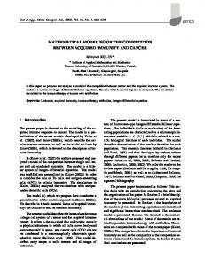
Climate and the Economy) model, arguably one of the simplest and most widely used global climate economy models ever developed. Climate modeling has also made its way into movies, the theme of the spectacular movie The Day After Tomorrow (Twentieth Century Fox, 2004) is about a climatologist who, through his modeling over global warming, has uncovered some startling news regarding the unexpected turnover of the Gulf Stream. Although the movie strongly exaggerate the possible speed with which the next Ice age is approaching, it gives an interesting view on how hard it is to get politicians and policymakers to understand the analyzing of complex and huge mathematical models. Global and regional models The fact that there exists so called weathercast service whose aim is to try to predict the weather of tomorrow from a large scale of different sources is well known among the most. Normally the weathercast service is not restricted to a country or a continent; instead the weathercast services are divided into regions (see figure 1). The weathercast SWECLIMs typical regional modeling area is shown in figure 1 below. Each regional weathercast service is divided into giant “pixels” or calculation squares. With a resolution of squares with a side length equal to 44 kilometers there are 114 × 82 horizontal calculation squares. Vertically between 19 to 24 levels up to a height of approximately 30 kilometers is used. Even if the area is just a small part f the surface of the earth, the resolution in the regional model implies that the number of calculation squares (e.g. 114 × 82 × 19 = 177 612) is comparable with the complexity in global models. Moreover, in every calculation square a number of variables are measured and calculated (temperature, moistness, wind, cloudiness, and so forth) with a time frequency between 5 to 30 minutes. In reality this exercise in calculations and measurements presuppose the access to super computers for both global and regional 100
Analyses
simulations (SWECLIM, 2006).
Figure 1: Weathercast region for calculation and simulation
Models on local heating Global and regional models for climate changes and weathercast service may very well be transformed into treatable models at a local level and thereby identified as another type of mathematical model, useful in a course on mathematical modeling and/or in the pre-service teachers’ future professional life as teacher. Consider the following situation: A rectangular house is to be built with exterior walls that are 2.40 meters high. One wall of the house will face north. The total enclosed area of the house will be 140 square meter. Annual heating costs for the house are determined as follows. Each square meter of exterior wall with a northern exposure adds 40 Euros to the annual heating cost; each square meter of exterior wall with an eastern or western exposure adds 20 Euros to the annual heating cost; each square meter of exterior wall with a southern exposure adds 10 Euros to the annual heating cost. Denote by L the length of each of the north and south facing walls, and by W the length of each of the east and west facing walls. Compose a mathematical model that expresses the total annual heating cost C in terms of L.
For what value of L is the annual heating cost minimized, and what is the annual heating cost for this choice of L? The values given for the heating costs per square meter can only be
Analyses
ZDM 2006 Vol. 38(2)
known approximately. How does the solution depend on the given values for the heating costs?
average year locations.
From the information given, C = 2.4(4L + 2W + 2W + L) = 12L + 9.6W. Since the area of the house is 140 square meter, LW = 140 so W = 140/L. Hence C = 12L + 9.6⋅140/L, with L > 0. By making a reasonably careful graph of C versus L, the annual heating costs are observed to be minimized at L = 10, which corresponds to an annual heating cost of about 250 Euros. See figure 2.
Models on cooling The inverse to heating is cooling and even if it is hard to perform realistic and real time data collections of heating experiment, it is quite easy to ask students to study cooling phenomena. They can for instance be asked to bring a cup of coffee back to class after lunch and given a thermometer from a chemistry lab, they can monitor the cooling of the coffee in the cup. From experimental observations it is known that (up to a “satisfactory” approximation) the surface temperature of an object changes at a rate proportional to its relative temperature. That is, the difference between its temperature and the temperature of the surrounding environment. This is what is known as Newton's law of cooling. A suitable mathematical model is not hard to find with the curve fitting tools of today, even though it requires quite some mathematical background to derive a correct formula, in order to understand why a damped exponential function is the best fit for the measured data set.
2500
y
2000
1500
1000
500
x
0 0
10
20
30
40
50
60
70
80
90
-500
Figure 2: Model of heating costs vs. length of northern wall.
One way to analyze the effects of the heating costs on the solution would be to assume that the specified values are in the correct proportion, so that the true heating costs always are 4p, 2p, and p respectively. The dependence of the solution on p could then be examined. There is always a trade-off between model accuracy and solvability. We could also investigate what would happen if the house for instance would be built in a North-west direction, i. e. a 45 degree declination from the northern direction. In reality, heating costs are always balanced against the installation of cavity wall insulation in countries with strong winters, as in Sweden. Consequently the models also become much more complicated to construct and evaluate, see for instance Lingefjärd & Holmquist (2001) for a discussion about such a model regarding the economical incentives for cavity wall insulation with respect to the
temperature
on
specific
Population models It would be hard to not mention biological models when discussing observations of nature. Mathematical models of predator-prey systems are considered to be amongst the oldest in ecology. The Italian mathematician Volterra is known to have developed his ideas about predation from watching the rise and fall of Adriatic fishing fleets. When fishing was good, the number of fishermen and fishing boats increased, drawn by the success of others. After some time the fish declined, perhaps due to over-harvest, and then the number of fishermen and fishing boats also declined. After some time, the cycle repeated. The Lynx and the Hare case which is often cited as an example of the inbuilt balance of nature is the relationship between the Canada lynx and its primary prey, the snowshoe hare. For over 300 years, the Hudson Bay 101
ZDM 2006 Vol. 38(2)
Company has been involved in the fur trade in Canada. Company records show that the number of snowshoe hare pelts bought tends to fluctuate in a ten-year cycle, as does the number of lynx. However, the changes in the lynx cycle tend to lag behind those of the hare by about a year. The Hudson Bay Company has kept records dating back to 1840. It appears that the hare population increases to a level where the available winter food supply is largely exhausted. At that point, the hare population suffers an increase in mortality among young hares and a decrease in the birth rate. With fewer hares, the vegetation begins to recover from overbrowsing.
Figure 3: Model of hare and lynx populations in Hudson Bay over time. Edelstein-Keshet, 1988, p. 218.
Figure 3 shows the numbers of predator (lynx) and prey (hare) pelts brought to the company by trappers over a 90-year period. Note that, from 1875 to 1905, changes in the number of lynx pelts sometimes precede changes in the number of hare pelts. It indicates that prey population density may depend equally strong or even stronger on its own food supplies than on predator numbers. Volterra concluded the following assumptions based upon what he observed in nature: 1 2 3
4
102
Prey grow in an unlimited way when predators do not keep them under control Predators depend on the presence of their prey to survive The rate of predation depends on the likelihood that a victim is encountered by a predator He growth rate of the predator population is proportional to food intake (rate of predation).
Analyses
Using the simplest set of equations consistent with these assumptions, Volterra wrote down the following model: dx = ax − bxy dt dy = −cy + dxy dt
where x and y represent prey and predator populations respectively; the variables can for example represent biomass or populations densities of the species. The parameters a, b, c, and d has to do with net growth and death rates for the species. Using this model leads into considerations over cycles, steady states, and stable cycles and reveals and massive amount of mathematical preparation needed for just a “simple” system like this. See EdelsteinKeshet, 1988, pp. 218 – 223, for a throughout discussion and further development of the Volterra equations. It should be noted that there is an enormous amount of predators in nature, all within a more or less steady balance with their prey. Without prey, the predator dies. The most dangerous predator of all does however not have big teeth, sharp claws, powerful muscles, or especially keen senses nevertheless it is capable of killing any other creature on earth, and time and again has managed to hunt whole species into extinction. This predator often fails in finding a steady balance with its prey. Instead of physical prowess, it relies upon its superior intelligence - and a pair of opposable thumbs - to conceive and create tools, weapons, and strategies that compensate for its physical shortcomings as a predator. The ultimate predator is the human race. Population models are very well suited to adapt to classroom exercises and they are also excellent to use to introduce the software tool Excel. When modeling population relations, one normally ends up in difference equations, also known as recurrence relations. These entities are illustrated in applications dealing with population growth, competition, and
Analyses
ZDM 2006 Vol. 38(2)
predation in ecological systems. Closely connected are sequences and series and the behavior of population models easily approaches to chaos. What is good with using Excel is that students in general seem to have at least a rudimentary knowledge about how to use the spreadsheet and how to manipulate data in cells. The very best with Excel, or any spreadsheet of today, is that it is fairly easy to build a model that relays on the initial values of just on or two cells, and thereby the students can easily test the behavior of the model by themselves. See figure 4, where a model for foxes and rabbits are simulated in Excel and where a fox family can have 1 kit per year, a pair of rabbits produces 12 bunnies, and a fox dines on 1 rabbit per week. Foxes and Rabbits 8000 7000 6000 5000 4000 3000 2000 1000 0 1
2
3
4
5
6
7
Figure 4: Model of simulated fox and rabbit populations with initial values foxes = 10 and rabbits = 122
In this simulation, the rabbits will vastly overcome the foxes in just a couple of years. What is devastating though, is that if we change the initial values for foxes to 11, or decrease the initial value for rabbits to 121, then the rabbits and consequently the foxes, will all be gone within 5 – 6 years. Harvesting models The harvesting of renewable resources is studied intensively, due to the human races inclination to ruin the resources in our greed, instead of limiting ourselves to an optimal harvest. Many fishing grounds collapse under over fishing and many animal species are in danger of extinction because of indiscriminate hunting.
Let us consider a population of animals with N representing the population at time t, of which an annual and constant harvest E is taken. It can be shown that a well suited model for this kind of problems is a so called logistic model (see for instance Dreyer, 1993, pp. 37 – 49) which models the change of N over time t under the conditions given by the constants b, s, α and E. If these values are known, the solution N(t) can be determined. dN = (b − sN ) N − E , N (0) = α dt
(t > 0)
However, under the circumstances of the harvesting methods of human race, we are more interested in the terminal value of N as t → ∞. The critical question at hand is whether the population N will die out in a finite period of time. If hopefully not, will N tend to a limit β when t → ∞? The terminal value of N is important to ecologists who guard against the extinction of animal or botanical species, but also to scientists in agriculture who try to control disease spread. Especially in the calculation and determining of fishing quotas, scientist try to select an value of E in such an way that the annual catch is as large as possible without diminishing the stock. The problem is then to determine the limit β as a function of E. Ways to do this and examples of authentic use of this model and alteration of the model when working on critical harvesting problems can be found in Dreyer (1993). Models that can show the sensitivity of a balance between eradication and inundation are quite easy to construct and evaluate in Excel. Sometimes they illustrate chaotic behavior, sometimes not, all depending on frame factors and circumstances. In figure 5 we see the output from a student created mathematical model which takes the following five parameters as input: The number of bunnies per rabbit and year: a ≤ 100 The number of kits per fox and year: b ≤ 10 The number of rabbits eaten per fox and year: c ≤ 500 103
ZDM 2006 Vol. 38(2)
Analyses
The number of foxes to begin with: d ≤ 20 The number of rabbits to begin with: e ≤ 1000 Rabbits
Fox- and rabbit populations
Foxes x 100
The number of individuals
1200 1000 800 600 400 200 0 1
21
41
61
81
101
Time/year
Figure 5: Model of simulated fox and rabbit population with a = 77, b = 6, c = 122, d = 13, and e = 450.
Even with only small changes for the parametric values, the behavior of the model can change dramatically. Not all models are so changeable, though. Everlasting models Some models can take meandering and mysterious ways and eventually show to be useful in applications that were not intended, invented or considered when they were first discovered. The Platonic bodies are five polyhedral with faces that are regular polygons. Even though Plato mentions them in his work Timaios, they are known to be mentioned far earlier by, among others, the Pythagoreans and the Neolithic people of Scotland who developed the five solids far earlier, in the Bronze Age 4000 - 750 BC.
harmonies in the skies, Johannes Kepler tried to relate planetary orbits with geometrical figures. The Platonic and Pythagorean components in Kepler's conception of celestial harmony, however mystical in origin, helped to lead him to the three principles of planetary motion now known by his name. The Platonic bodies were considered to be equated to the four elements, with the tetrahedron equated with the “element” fire, the cube with earth, octahedron with air, and icosahedra with water. Plato considered the dodecahedron to be equated to the universe, but it was later associated with the ether. Archimedes (around 250 BC.) allowed himself to make models of the situation that occurs when two different sidoytor are allowed to connect, instead of just one type of sides. Archimedes found 13 such half regular bodies. One of them is the normal (soccer) football which is limited by 12 pentagons and 20 hexagons. Leonardo Vinci later constructed a geometrical model of that very body, see figure 6.
Figure 6: The Football polyhedron, by Leonardo da Vinci.
In the 18th century, Leonhard Euler proved that there are only five bodies with the quality that all faces should be regular polygons. The five Platonic bodies are: Tetrahedron 4 equilateral triangles Hexahedron (cube) 6 squares Octahedron 8 equilateral triangles Dodecahedron 12 pentagons Icosahedra 20 equilateral triangles
More than 2 thousand years after Archimedes modeling with half regular bodies, in the year 1985, three chemists discovered that a carbon molecule consisting of 60 carbon atoms, surprisingly was built according to this very polygon with a carbon atom in every corner. Since an American architect, Buckminster Fuller, used similar structures for his dome constructions, the chemist called their finding and similar carbon clusters for ”fullerenes”.
Sustained by a vision of mathematical
In October 1996, the three chemists Smalley,
104
Analyses
Curl and Kroto received the Nobel Prize for their discoveries of the famous Carbon-60ball, shaped like a soccer ball (12 pentagonal faces, 20 hexagonal faces, and 60 vertices). See figure 7.
Figure 7: A model of a carbon ball.
There are a number of other fullerenes in addition to C60, including C70, C74, and C82. The first transistor to be fashioned from a single “buckyball” - a C60 – was reported by scientists from the University of California at Berkeley in 2000. Research on fullerenes has further led to the discovery of a related type of carbon allotrope – nanotubes. In a nanotube the fullerenes the system of carbon balls on a sheet can be seen as tooled into a cylinder (see Petrucci, Harwood, & Heering, 1993, p. 506). Nanotubes possess unusual properties that offer the promise of applications in the macroscopic world and even more in the submicroscopic world of nanotechnology. Nanotubes might, for example, be useful for channel molecules into the interior of cells. This modeling structure is an astonishing example of a models journey over time, a model that circumscribes our lives in different ways over the millenniums. Even though the modeling journey for the Platonic bodies normally creates interest and discussions among the students, at the same time they normally realize and agree about the fact that this modeling area goes beyond the natural
ZDM 2006 Vol. 38(2)
boundaries of a 10-week course. Medical models The fact that medical treatment becomes more and more advanced and technical is something many of us witness. The numbers of mathematical models used in medicine, either for measuring and treatment, or for research and analyzes, seems to be unlimited. Students are in general undefined aware of the use of mathematics and technology in general and advanced hospital care through experiences with relatives and/or friends. Mathematical modeling within the field of medical treatment is also something that very well may be used in courses for teacher education programs. Body temperature All grown ups have taken somebody’s body temperature some time, either our own temperature when feeling feverish, or our kids or some other relative’s temperature. Basically that measurement principle corresponds with a very simple model for body temperature. Humans, like mammals and birds, are homeothermic and control their central body temperature within a relatively narrow range despite a wide range of environmental temperature. In humans, the range is normally 37 ± 0.5 ºC. A constant temperature is essential, as variation in temperature may bring about changes in enzyme reactions rates governing physiological processes and some metabolic processes could not occur if body temperature were allowed to cool to the temperature of the environment. Slight variation in body temperature, however, does not occur naturally in man. There is a circadian or diurnal rhythm of around 0.4 ºC, the temperature being lowest in the early morning and reaching maximum in the early evening. There is also a small variation in body temperature during the menstrual cycle in women. If looking at a model of the human body, we define the central core of the body which is 105
ZDM 2006 Vol. 38(2)
maintained at the constant temperature, and the shell or surface layer of the body, with a lower, more variable temperature which can range from 32 to 35 ºC depending on physiological factors. See figure 8.
Analyses
with movement. Medications control symptoms primarily by increasing the levels of dopamine in the brain. One such medicine is L-dopa. Table 1 illustrates the levels of Ldopa in the blood, in nanograms per milliliter, as a function of time, in minutes after the drug is administered in the body. See Table 1. Table 1: Data set over L-dopa accumulation in body
Time (minutes) 0 20 40 60 80 100 120 140 160 180 200 220 240 300 360
Figure 8: Model of the human body and temperature zones. Davis, Parbrook, & Kenny, 1995, p. 120.
The central core includes the brain, thoracic and abdominal organs and also some of the deep tissues of the limbs, the amount varying with the environmental temperature as represented by the intermediate zone. The shell is a layer with a variable depth of around 2.5 cm. The temperature in the body core depends on the balance between heat production in the core and heat loss through the shell or surface layer. Instead of using core temperature alone, a formula for combining core and average skin temperature is used to give the average patient temperature: Average patient temperature = 0.66 × Core temperature + 0.34 × average skin temperature. We see that in the formula it is assumed that two-thirds of the heat is in the core and onethird in the shell area. For example, if the core temperature is 37 ºC and the average skin temperature is 34 ºC, then the average patient temperature is 36 ºC. Modeling Drug Responses Parkinson's disease is a disorder of the brain characterized by shaking (tremor) and difficulty with walking, movement, and coordination. The disease is associated with damage to a part of the brain that is involved 106
L-dopa (nanograms per milliliter) 0 300 2700 2950 2600 1550 1100 900 725 600 510 440 300 250 225
A quick sketch of the process illuminates the hidden behavior of any medical treatment, regardless of how we obtain the drug and for what purpose. After some delayed peak in our system, the drug decrease and evidentially vanish. See figure 9. L-dopa (nanograms per milliliter)
4000 3000 2000 1000 0 0
50
100
150
200
250
300
350
400
Time (minutes)
Figure 9: Graphical representation of the data set in Table 1.
Students can be asked to invent their own questions in connection with the drug response data set. I have quite successfully tried this exercise with students, and their responses are in general the same as I would have asked myself: When does the peak
Analyses
occur? How high is the L-dopa concentration in the blood then? What kind of mathematical model fits the data set best? When will the concentration of L-dopa go under some decided limit, which equals to the concept of being “drug-free” in this situation? Cardiac Output Measurement The main organ in the thoracic region is the heart. The function of the heart is to pump blood throughout the body. The blood carries oxygen (O2) from the lungs to the various tissues of the body and carries carbon dioxide (CO2) from the tissues back to the lungs. In constructing a mathematical model of the circulatory system in a human body, we consider it to be a closed loop and assume that the blood flowing around this loop is incompressible. Consequently, the total volume V of blood (measured in liters) in the system is constant. The rate at which this blood flows around the circulatory loop is critical. We can (in principle) measure the flow rate (in liters/minute) past any given point in the system. Attention ordinarily is focused on the heart itself, and the cardiac output CO is the rate at which blood is pumped out of the heart. The cardiac output of the heart is the product of •
the stroke volume SV -- the volume of blood pumped per beat -- and
•
the heart rate HR -- number of beats per minute.
Cardiac output is often monitored during and after surgery (especially in the case of heart surgery). Serial measurements are used to assess the general status of the circulation and to determine the appropriate hemodynamic therapy and estimate its efficacy. Several other useful variables—such as the stroke volume, the left ventricular stroke work index, the systemic vascular resistance, and the stroke index—can be determined once the cardiac output is known. Cardiac output can be measured by several techniques, all based on the same idea for
ZDM 2006 Vol. 38(2)
measuring the flow rate in a fluid loop. A measurable indicator is injected into the fluid, and its subsequent concentrations at various points in the flow loop are measured. Such a method was first proposed in 1870 by the German physiologist Adolph Fick, who described a means of determining blood flow by measuring overall oxygen intake and content in the blood. One determines how much oxygen an animal takes out of the air in a given time…. During the experiment one obtains a sample of arterial and a sample of venous blood. In both the content of oxygen is to be determined. The difference in oxygen content tells us how much oxygen each cubic centimeter of blood takes up in its course through the lungs, and since one knows the total quantity of oxygen absorbed in a given time, one can calculate how many cubic centimeters of blood passed through the lungs in this time. (Miller, 1982, p. 1058)
The indicator dilution method is a variant of Fick's technique in which a known amount I of an indicator substance is injected into the blood stream and its concentration C(t) (in liters per cubic meter) is measured as a function of time t at a single downstream location. This dilution method was first introduced by the British physician Stewart, who together with a colleague Hamilton, developed the dye solution method and the Stewart-Hamilton formula: CO =
I ∞
∫ C(t ) dt 0
which gives the corresponding cardiac output CO. (See Glantz, 1979, p. 38; Miller, 1982, p. 1059.) For a throughout derivation of this formula and its history, see Lingefjärd (2002). Complications in the Model It should be noted that today the dye solution method has been almost entirely replaced by variants of a thermodilution method. Originally (around 1954), the thermodilution method used an iced or room temperature solution of salt or dextrose in water. Today, the method uses a small heating thermistor on the Swan-Ganz catheter (a lung artery 107
ZDM 2006 Vol. 38(2)
catheter). The temperature TB(t) of the blood at the sensor is measured, and the StewartHamilton formula discussed above is replaced with the formula (Miller, 1982, p. 1059): CO =
KI (TB − TI ) ∞
∫ T (t ) dt B
0
where TB – TI = initial blood-injectate temperature difference (TB = TB(0)), and K = an empirical constant depending on the catheter size, specific heat and volume of the injectate, and the rate of injection. A significant complication results from the fact that the circulatory system is a closed loop. Before the indicator concentration curve returns to zero (i.e., when the entire indicator has passed the censor), the indicator concentration exhibits a secondary peak due to recirculation. There are two ways to evaluate cardiac output in the presence of recirculation. One could develop theoretical equations to account explicitly for recirculation, but this approach would require detailed analysis of the indicator washout curve, rather than simply finding the area under the curve. A simpler and perhaps more effective method to account for recirculation is to remove its effect from the observed indicator “washout curve.” It can be shown (see Lingefjärd, 2002) that the initial “downstroke” is a straight line on a semi-log plot. With the help of suitable software or graphing calculators, we may use measured values of the concentration to fit an exponential curve to the washout part (to the right of the peak) of the curve in Figure 10.
Figure 10: Plot of a washout curve on a semilogarithmic paper. Davis, Parbrook, & Kenny, 1995, p. 67. 108
Analyses
All together, both the basic and more advanced Stewart-Hamilton formula, gives a glimpse of how much beautiful mathematics that lies underneath treatment methods in our hospitals and how wonderfully many different methods from upper secondary curriculum comes together in this theory: logarithms, calculus, differential, equations, numerical methods, and so forth. Models in Sports The step from health care to physical training and health should not be too odd. There are of course many mathematical models for measuring, analyzing and improving results for any field in sports. I will give an example of a model used to illustrate the difficult task of judging performance in sports on a technical and artistic level. This is regularly demanded in sports like gymnastics, figure skating and diving. We know how to measure height, length, weight, and speed – but how do we measure artistry, beauty, or creativity? The short program in ice skating is given two marks, one for required elements and one for presentation. Normally the judges keep count of the errors and subtract a value between 0.1 and 1 out of total number of marks for the required elements. The second mark (normally the same maximum) is given for the general impression made by the composition of the program, artistic quality, harmony of music and motion, and so on. Normally the judges work in a panel with other experts. It can be assumed that in a panel of n members, each member comes with a subjective (opportunistic) and one objective opinion. Two such different opinions can exist practically indisputable. Any sports judge forms an “objective” estimate of an athlete’s ability, at the same time as the fact that the judge represents a country, a certain school (trend), and a certain sports society, makes the judge biased. Let us suppose that a judge always states a relation somewhere between his objective and his subjective opinion. Let us call them Ro and Rs. Consider a situation, where a judge gives a skater two marks, one for technical merit and
Analyses
one for artistic impression, and where the maximum mark is six. The place or position the judge gives the skater is determined by the sum of these two marks. Assume that the relation Ro = (5.7; 5.8) expresses the judge’s objective opinions and the relation Rs = (5.0; 5.7) expresses the judge’s subjective opinion. Then pairs of marks with a sum more than 10.7 and less than 11.5 will form a set of relations lying between Ro and Rs. This area of possible outcomes is illustrated in figure 10 and can be algebraically expressed by x + y ≤ 11.5 x + y ≥ 10.7 0≤x≤6 0≤y≤6
ZDM 2006 Vol. 38(2)
coverage, since most people like to or even require being able to connect with their cellular telephones anywhere and everywhere. When modeling the objective to get as much coverage as possible in the landscape, the mobile operators companies need to use geometry. Using a geometrical model, it permits us to choose between different shapes in basic geometry. We can for instance compare between hexagons and circles to represent cells and ask us which one that is the most suitable (see figure 11)?
Figure 12: Placing communication antennas according to geometrical shapes.
Figure 11: A Linear Programming model of how to judge ice skating performance. Sadovskii & Sadovskii, 1993, p. 46.
Models in communication The world is transforming into a connected world with possibilities to communicate everywhere. Basically, it is built upon the presence of a cellular radio which provides mobile telephone service by employing a network of cell sites distributed over a wide area. A cell site further contains a radio transceiver and a base station controller which manages, sends, and receives traffic from the mobiles in its geographical area to a cellular telephone switch. It also employs a tower and its antennas, and provides a link to the distant cellular switch called a mobile telecommunications switching office. This office places calls from land based telephones to wireless customers, switches calls between cells as mobiles travel across cell boundaries, and authenticates wireless customers before they make calls. The keyword in general is
Any cellular system will in reality have gaps in coverage, but the hexagonal shape allows us to more neatly visualize, in theory, how the system could be laid out. Notice how the circles in figure 8 would leave gaps in our layout. Still, one might ask why hexagons and not for instance triangles or rhomboids? The answer has to do with frequency planning and vehicle traffic and the inbuilt genius of nature. After much experimenting and calculating, the Bell team came up with the same solution that the honeybee has known about all through history. The central feature of the bee hive is the honeycomb which can be modeled as the hex system. Using 3 sectored sites, major roads could be served by one dominant sector, and a frequency re-use pattern of 7 could be applied that would allow the most efficient re-use of the available channels. See figure 13.
109
ZDM 2006 Vol. 38(2)
Analyses Area (Triangle ABC)= 13,87 square cm Area(Hexagon) = 1,39 square cm (Area (Triangle ABC))/Area(Hexagon) = 10,00 A
B
Figure 13: The connection between site antennas for mobile telephoning coverage and the honeybee’s honeycomb.
Note how neatly seven hexagon shaped cells fit together, and try to perform that with a triangle. Clusters of four and twelve are also possible but frequency re-use patterns based on seven are most common. I have found it useful to introduce this geometrical existence in today’s communication before I introduce geometrical modeling problems. One of the most interesting of a variety of geometrical modeling problems is the following, since it also connects to a more “common” mathematical modeling process at the end. Models in geometry Walter’s theorem was first presented as Marion Walter’s theorem in the November 1993 issue of the Mathematics Teacher in the section called Readers Reflections (Cuoco, Goldenberg, and Mark 1993). In short it says the following, modeled by The Geometer’s Sketchpad and illustrated by figure 14: If the trisection points of the sides of any triangle are connected to the opposite vertices, the resulting hexagon has area onetenth the area of the original triangle.
110
C
Figure 14: Walter’s theorem In the May 1996 issue of the Mathematics
Teacher in an article called Morgan’s theorem (Watanabe, Hanson, and Nowosielski 1996), a ninth grader Ryan Morgan was interested in finding out what would happened if the sides of the triangles were partitioned into more than three congruent segments. According to the article, Ryan and his teacher called the process of dividing a side of a triangle into n congruent segments “n-secting”, and using the Geometer’s Sketchpad, Ryan experimented with different n-sections (Watanabe et. al., p. 420). The article further explains the methodology of Ryan’s investigations and what it led to – not surprisingly Ryan was invited to present his conjecture at a special mathematics colloquium at Towson State University in 1994. A throughout discussion about the way my students handled Walter’s – Ryan’s problem can be found in Lingefjärd & Holmquist (2003). Students’ reactions During the years, I have tried to monitor students’ reactions and opinions about several different approaches to mathematical modeling and different problem situations. This is also in line with university policy in Sweden, that every course should be evaluated against students’ experiences and opinions. The distribution of the more than 200 responses I have recorded are illustrated in figure 15. No doubt that medicine is
Analyses
ZDM 2006 Vol. 38(2)
something we all can connect to regardless where we are in life. Students' ratings
Geometry
Topic
Heating - cooling Medicine Populations Sports 0
0,1
0,2
0,3
0,4
Percent
Figure 15: Student’s opinions about modeling areas
Students have argued that models in geometry are “fun”, heating and cooling is interesting and “useful”, but models in medicine are “real” in some overall sense and that fact seems to have given the modeling process some extra energy for many students. I chose the two following excerpts from different course evaluations: The modeling problem about the drug response really turned me on; right now I cannot watch a person taking a headache pill without thinking about the peak of concentration in the blood, followed by a slowly declining curve, approaching the x-axis. My mother is a doctor and the fact that I, her youngest son, could tell her something about cardiac output which she didn’t know is fantastic! Not only did I teach her basic medicine facts, I also showed her how important mathematics is in her profession. I loved it!
Well, to be honest – which model area do you prefer, dear reader? I assume many of us feel closely connected to mathematical models in medicine, since we know we will be part of some of them mentioned in this article on day or another. Conclusions For most people, the value of mathematics most likely lies in applications, and modeling is one of the main and most useful applications of mathematics. Prospective mathematics teachers are just the same as the
general public in that respect, they like to know the specific value of what courses they take. In the modeling process, one may use mathematical equations, spreadsheets, curve fitting tools, computer simulations, or physical replicas. Not all methods or forms of mathematical modeling are applicable to all problems, but each validated model gives insight into how the system under study works. It is difficult to teach mathematical modeling in traditional ways, and the importance of mathematical modeling within the mathematics curriculum is well recognized, and seemingly growing. To teach courses in mathematical modeling do not only offer opportunities to discuss and teach the importance of modeling cycles, curve fitting techniques, evaluation of models and limitations of prediction, but also the existence of mathematics in our everyday life. References Blum, W., & Niss, M. (1989). Mathematical problem solving, modelling, applications, and links to other subjects – state, trends and issues in mathematics instruction. In W. Blum, M. Niss, & I. Huntley (Eds.), Modelling, applications and applied problem solving: Teaching mathematics in a real context (pp. 121). London: Ellis Horwood. Blum, W. (1991). Applications and modelling in mathematics teaching – a review of arguments and instructional aspects. In M. Niss, W, Blum & I. Huntley (Eds.), Teaching of mathematical modelling and applications (pp. 10-29). London: Ellis Horwood. Clayton, M. (1999). Industrial applied mathematics is changing as technology advances. In C. Hoyles, C. Morgan, & G Woodhouse (Eds.), Rethinking the mathematics curriculum (pp. 22-28). London: Falmer. Cuoco, A., Goldenberg, P., & Mark, J. (1993). Reader reflections: Marion’s theorem. Mathematics Teacher 86(8), 619. Davis. P. D., Parbrook, G. D., Kenny, G. N. C. (1995): Basic Physics and Measurement in Anaesthesia. Oxford: Butterworth Heinemann. Dreyer, T. P. (1993). Modelling with Ordinary Differential Equations. Boca Raton, Florida: CRC Press Inc. 111
ZDM 2006 Vol. 38(2)
Lingefjärd, T. (2002). Mathematical modeling for preservice teachers: A problem from anesthesiology. The International Journal of Computers for Mathematical Learning 7(2), pp. 117–143. Lingefjärd, T. & Holmquist, M. (2001). Mathematical modeling and technology in teacher education - Visions and reality. In J. Matos, W. Blum, K. Houston, S. Carreira (Eds.) Modelling and Mathematics Education ICTMA 9: Applications in Science and Technology (pp. 205-215). Horwood: Chichester. Lingefjärd, T. & Holmquist, M. (2003). Learning mathematics using dynamic geometry tools. In S. J. Lamon, W. A. Parker, S. K. Houston (Eds.), Mathematical Modelling: A Way of Life. ICTMA 11 (pp. 119-126). Horwood: Chichester. Meadows, D.H., Richardson, J. and Bruckmann, G.. (1982). Groping in the Dark: The First Decade of Global Modeling. Chichester: John Wiley & Sons. National Council of Teachers of Mathematics. (1998). Principles and standards for school mathematics: Discussion draft. Reston, VA: Author. Niss, M. (1989). Aims and scope of mathematical modelling in mathematics curricula. In W. Blum, J. Berry, R. Biehler, I. Huntley, R. Kaiser-Messmer & K. Profke (Eds.), Applications and modelling in learning and teaching mathematics (pp. 22-31). Chichester: Ellis Horwood. Petrucci, R. H., Harwood, W. S. & Herring, F. G. (2002). General Chemistry Principles and Modern Applications, Eighth Edition. New Jersey: Prentice Hall. Sadovskii, L. E., & Sadovskii, A. L. (1993). Mathematics and Sports. The American Mathematical Society: Edelstein-Keshet, L. (1988). Mathematical Models in Biology. New York: McGraw Hill. Skolverket. (1997). Kommentar till grundskolans kursplan och betygskriterier i matematik. [Commentary to the Swedish comprehensive school curriculum]. Stockholm: Liber distribution. Skolverket. (2006). Förslag till kursplan [Curriculum proposal] 2006-01-31, Dnr 612004:2637. Stockholm: Liber distribution. SWECLIM. (2006). http://www.smhi.se/hfa_coord/ sweclim_bild _ark/ oversikt1/oversikt1.htm Swetz, F., & Hartzler, J., S. (1991). Mathematical modeling in the secondary school curriculum. 112
Analyses
The National Council of Teachers of Mathematics: Reston, Virginia. Watanabe, T., Hanson, R., & Nowosielski, F. (1996). Morgan’s theorem. Mathematics Teacher 89(5), 420-423. ______________
Author Thomas Lingefjärd, Associated Professor, Department of Mathematics Education, University of Gothenburg, and Department of Mathematics and Mathematics Education, University of Jonkoping, Sweden. E-mail:
[email protected]