cle if and only if T is a caterpillar, i.e., it is a single path with several leafs connected to it. Our first main result is a simple graph-theoretic characterization of trees ...
Hamiltonian paths in the square of a tree Jakub Radoszewski1 and Wojciech Rytter1,2? 1
Department of Mathematics, Computer Science and Mechanics, University of Warsaw, Warsaw, Poland [jrad,rytter]@mimuw.edu.pl 2 Faculty of Mathematics and Informatics, Copernicus University, Toru´ n, Poland
Abstract. We introduce a new family of graphs for which the Hamiltonian path problem is non-trivial and yet has a linear time solution. The square of a graph G = (V, E), denoted as G2 , is a graph with the set of vertices V , in which two vertices are connected by an edge if there exists a path of length at most 2 connecting them in G. Harary & Schwenk (1971) proved that the square of a tree T contains a Hamiltonian cycle if and only if T is a caterpillar, i.e., it is a single path with several leafs connected to it. Our first main result is a simple graph-theoretic characterization of trees T for which T 2 contains a Hamiltonian path: T 2 has a Hamiltonian path if and only if T is a horsetail (the name is due to the characteristic shape of these trees, see Figure 1). Our next results are two efficient algorithms: linear time testing if T 2 contains a Hamiltonian path and finding such a path (if there is any), and linear time preprocessing after which we can check for any pair (u, v) of nodes of T in constant time if there is a Hamiltonian path from u to v in T 2 . Keywords: tree, square of a graph, Hamiltonian path
1
Introduction
Classification of graphs admitting Hamiltonian properties is one of the fundamental problems in graph theory, no good characterization of hamiltonicity is known. There are multiple results dealing with algorithms for finding Hamiltonian cycles in particular families of graphs, see e.g. [2]. The k-th power of a graph G = (V, E), denoted as Gk , is a graph over the set of vertices V , in which the vertices u, v ∈ V are connected by an edge if there exists a path from u to v in G of length at most k. The graph G2 is called the square of G, while G3 is called the cube of G. Hamiltonian cycles in powers of graphs have received considerable attention in the literature. The classical result in this area, by Fleischner [3], is that the square of every 2-connected graph has a Hamiltonian cycle, see also the alternative proofs [2, 4, 12]. Afterwards Hendry & Vogler [7] proved that every connected S(K1,3 )-free graph has a Hamiltonian square (where S(K1,3 ) is the subdivision ?
The author is supported by grant no. N206 566740 of the National Science Centre.
2
J. Radoszewski, W. Rytter
graph of K1,3 ), and later Abderrezzak et al. [1] proved the same result for graphs satisfying a weaker condition. As for the cubes of graphs, Karaganis [8] and Sekanina [10] proved that G3 is Hamiltonian if and only if G is connected. Afterwards, Lin & Skiena [9] gave a linear time algorithm finding a Hamiltonian cycle in the cube of a graph. The analysis of Hamiltonian properties of squares of graphs was also extended to powers of infinite graphs (locally finite graphs), see [5, 10, 11]. In this paper we consider Hamiltonian properties of powers of trees. Harary & Schwenk [6] proved that the square of a tree T has a Hamiltonian cycle if and only if T is a caterpillar, i.e., it is a single path with several leafs connected to it. On the other hand, the k-th power of every tree is Hamiltonian for any k ≥ 3 [9, 10]. However, there was no previous characterization of trees with squares containing Hamiltonian paths. We introduce a class of trees T , called here (u, v)-horsetails, such that T 2 contains a Hamiltonian path connecting a given pair of nodes u, v if and only if T is a (u, v)-horsetail. We provide linear time algorithms finding Hamiltonian paths in squares of trees.
2
Caterpillars and horsetails
We say that P is a k-path in G if P is a path in Gk , similarly we define a kcycle. Additionally define a kH-path and a kH-cycle as a Hamiltonian path and a Hamiltonian cycle in Gk respectively. If Gk contains a kH-cycle (a kH-path respectively) we call G k-Hamiltonian (k-traceable respectively). A tree T is called a caterpillar if the subtree of T obtained by removing all the leafs of T is a path B (possibly an empty path). A caterpillar is called non-trivial if it contains at least one edge. We call the path B = (v1 , . . . , vl ) the spine of the caterpillar T . By Leafs(vi ) we denote the set of leafs connected to the node vi . A tree has a 2H-cycle if and only if it is a caterpillar [6], see Fig. 5. We proceed to the classification of 2-traceable trees. Let T be a tree and let u, v ∈ V be two of its nodes, u 6= v. Let P = (u = u1 , u2 , . . . , uk−1 , uk = v) be the path in T connecting u and v. We call the nodes in P the main nodes, and the neighbors of the nodes in P from the set V \ P are called secondary nodes. By Layer (ui ), i = 1, . . . , k, we denote the connected component containing ui in T \ (P \ {ui }). Each main node ui for which Layer (ui ) is a caterpillar can be classified as: type A: at most one component of Layer (ui ) \ {ui } is a non-trivial caterpillar type B: exactly two components of Layer (ui ) \ {ui } are non-trivial caterpillars free node: Layer (ui ) \ {ui } is empty. In other words, ui is a type A node if ui is an endpoint of the spine of the caterpillar Layer (ui ) or a leaf adjacent to the endpoint of the spine. The node ui is a type B node if ui is an inner node of the spine of the caterpillar Layer (ui ). Also note that every free node is a type A node.
Hamiltonian paths in the square of a tree
3
Fig. 1. An example (u, v)-horsetail. White squares represent type B nodes, black squares represent free nodes. The nodes u and v are the leftmost and rightmost nodes on the horizontal path (the main path), they are also free nodes (in this example, in general case they can be non-free).
By ui1 , ui2 , . . . , uim , 1 ≤ i1 < i2 < . . . < im ≤ k, we denote all the type B nodes in T , additionally define i0 = 0 and im+1 = k + 1. The tree T is called a (u, v)-horsetail if (?) every main node ui is a type A or a type B node, and (??) for every j = 0, . . . , m, at least one of the nodes uij +1 , uij +2 , . . . , uij+1 −1 is a free node. A tree is a horsetail if it is a (u, v)-horsetail for some u, v. The condition (??) can also be formulated as follows: – – – –
between any two type B nodes in P there is at least one free node, and there is at least one free node located before any type B node in P , and there is at least one free node located after any type B node in P , and there is at least one free node in P .
In particular, the nodes u1 and uk must be type A nodes. See Fig. 1 and 2 for examples of horsetails and trees which are not horsetails. In the next section we show that T contains a 2H-path connecting the nodes u and v if and only if T is a (u, v)-horsetail, see also Fig. 3. We present a linear time algorithm finding a 2H-path from u to v in a (u, v)-horsetail. Afterwards, in Section 4 we provide a linear preprocessing time algorithm which enables constant time queries for existence of a 2H-path from u to v. We also obtain a linear time test if T is 2-traceable.
3
2H-paths in (u, v)-horsetails
In this section we describe a linear time algorithm finding a 2H-path from u to v in a (u, v)-horsetail. We then show that a tree contains a 2H-path from u to v if and only if it is a (u, v)-horsetail.
4
J. Radoszewski, W. Rytter
(a) u
A
(c) u
A
v A
A,f
B
A,f
A
A
A
A
A
B
A
A,f
B
A,f
(b)
u A,f
v A
v
(d) u
v
A
A
A,f
A,f
A,f
Fig. 2. (a) and (b): The main paths (P ) of example horsetails; A, B and f denote a type A node, type B node and a free node respectively. (c) and (d): The main paths of example trees which are not (u, v)-horsetails.
2
6
3
5
13
7
10
9 8
1
4
20 15
19
25
18
21
24
12
16
23
11
17
22
14
26
Fig. 3. The tree without the unlabeled nodes is a (1, 26)-horsetail having a 2H-path 1, 2, 3, . . . , 26. If any of the unlabeled nodes is present in the tree, the tree is not a (1, 26)-horsetail and does not contain any 2H-path from 1 to 26.
For a 2-path S, by first(S) and last(S) we denote the first and the last node in S. Let S be a 2H-path from u to v in a (u, v)-horsetail T . We say that S is a layered 2H-path if the nodes of T are visited in S in the order of the subtrees Layer (ui ), i.e., first all the nodes of Layer (u1 ) are visited in some order, then all the nodes of Layer (u2 ) etc. Then we can divide S into parts (S1 , S2 , . . . , Sk ), such that every Si contains only nodes from Layer (ui ). Note that, for any i, each of the nodes first(Si ), last(Si ) is either a main node or a secondary node. The following algorithm 2H-path-horsetail finds a layered 2H-path in a (u, v)horsetail T , see Fig. 4. Informally, the algorithm works as follows. In each layer Layer (ui ) a 2H-path Si is found, using an auxiliary routine 2H-path-caterpillar (Layer (ui ), first, last), and appended to the constructed 2Hpath S. The algorithm constructs the 2H-path in a greedy manner: for each i,
Hamiltonian paths in the square of a tree
5
last(Si ) = ui , if only this is possible to achieve. If so, we say that after the i-th layer the algorithm is in the main phase, otherwise it is in the secondary phase. In the algorithm we use auxiliary functions: – any-secondary-node(Layer (w)), which returns an arbitrary secondary node from the layer Layer (w); – a-secondary-node-preferably-leaf (Layer (w)), which finds a secondary node being a leaf in Layer (w), if such a secondary node exists, and any secondary node from this layer otherwise; – another-secondary-node(Layer (w)), which returns a secondary node from Layer (w) different from the secondary node returned by the previous asecondary-node-preferably-leaf (Layer (w)) call.
Algorithm 2H-path-horsetail(T, u, v) 1: 2: 3: 4: 5: 6: 7: 8: 9: 10: 11: 12: 13: 14: 15: 16: 17: 18: 19:
Compute the main nodes u1 , . . . , uk and the layers Layer (u1 ), . . . , Layer (uk ); first := u1 ; if free(u1 ) then last := u1 else last := any-secondary-node(Layer (u1 )); S := 2H-path-caterpillar(Layer (u1 ), first, last); for i := 2 to k do w := ui ; if w is a free node then first := last := w; else if last is a secondary node then first := w; last := a-secondary-node-preferably-leaf(Layer (w)); else first := a-secondary-node-preferably-leaf(Layer (w)); last := w; if 2H-path-caterpillar(Layer (w), first, last)=NONE then last := another-secondary-node(Layer (w)); S := S+2H-path-caterpillar(Layer (w), first, last); return S;
Fig. 4. Finding a 2H-path in a horsetail in linear time.
Let us investigate how the algorithm works for respective types of nodes ui . We have first(S1 ) = u1 ; the 2-path S1 ends in a secondary node in Layer (u1 ) if only u1 is not free. Otherwise, obviously, last(S1 ) = u1 . Hence, after Layer (u1 ) the algorithm is in the main phase only if u1 is free. Afterwards, whenever ui is a free node, we simply visit it, with first(Si ) = last(Si ) = ui . Hence, after any free node the algorithm switches to the main phase.
6
J. Radoszewski, W. Rytter
Otherwise, if ui is a type A node, we have two cases. If the algorithm was in the main phase then we can choose any secondary node for first(Si ) and finish the 2H-path in Layer (ui ) in last(Si ) = ui — this is the desired configuration. On the other hand, if last(Si−1 ) is a secondary node, then we must have first(Si ) = ui and we finish in a secondary node. Thus, visiting a non-free type A node does not alter the phase of the algorithm. Now let ui be a type B node. Due to the (??) condition of the definition of a horsetail, before entering Layer (ui ) the algorithm is in the main phase. Thus we can choose first(Si ) as a secondary node. There is no 2H-path Si ending in ui in this case (the proof follows), therefore last(Si ) is another secondary node in Layer (ui ). Hence, a type B node changes the main phase into the secondary phase. Finally, if uk is a free node then first(Sk ) = last(Sk ) = uk and this ends the path S. Otherwise, we must have last(Sk ) = uk , hence first(Sk ) must be a secondary node and after the (k − 1)-th layer the algorithm must be in the main phase. This is, however, guaranteed by the (??) condition of the definition of a horsetail (see also the alternative formulation of the condition). Thus we obtain the correctness of the algorithm provided that the requested 2H-paths in the caterpillars Layer (ui ) exist. We conclude the analysis with the following Theorem 1. In its proof we utilize the following auxiliary lemma, we omit its proof in this version of the paper. Lemma 1. Every 2H-cycle in a caterpillar with the spine B = (v1 , . . . , vl ), l ≥ 1, and the leafs Leafs(v1 ), . . . , Leafs(vl ), has the form v1 P2 v3 . . . vl−1 Pl vl Pl−1 . . . P3 v2 P1
for 2 | l
v1 P2 v3 . . . Pl−1 vl Pl vl−1 . . . P3 v2 P1
for 2 - l
where Pi , for i = 1, . . . , l, is an arbitrary permutation of the set Leafs(vi ).
1
3
7
5
1
3
9
5
7
2
8
4
6
2
10
4
8
6
Fig. 5. To the left: a 2H-cycle 1, 2, . . . , 8 in a caterpillar with the spine 1–3–7–5 of even length. To the right: a 2H-cycle 1, 2, . . . , 10 in a caterpillar with an odd spine 1–3–9–5–7.
Theorem 1. Assume that T is a (u, v)-horsetail. Then the algorithm 2H-pathhorsetail(T, u, v) finds a layered 2H-path from u to v in linear time.
Hamiltonian paths in the square of a tree
7
Proof. It suffices to prove that the 2H-path-caterpillar procedure returns the 2H-paths as requested, depending on the type of the node ui . If ui is a type A node (in particular, if i = 1 or i = k) then the arguments of the 2H-path-caterpillar call are ui and a secondary node in Layer (ui ). In this case, ui is either an endpoint of the spine of the caterpillar Layer (ui ) or a leaf of Layer (ui ) connected to an endpoint of the spine. Let v1 , . . . , vl be the spine nodes of Layer (ui ); we assume that l > 0, since otherwise the conclusion is trivial. Thus, we are looking for a 2H-path in Layer (ui ) connecting the nodes v1 and w for some w ∈ Leafs(v1 ), or the nodes vl and w for some w ∈ Leafs(vl ). Note that we could also have the pair of nodes v1 and v2 or vl−1 and vl here, however these cases are eliminated in the algorithm by choosing a-secondary-node-preferablyleaf. Equivalently, we are looking for a 2H-cycle in Layer (ui ) containing an edge between the nodes v1 and w or vl and w. By Lemma 1, for any w ∈ Leafs(v1 ) (w ∈ Leafs(vl ) respectively) there exists a 2H-cycle in Layer (ui ) containing the edge v1 w (vl w respectively), and this 2H-cycle can be found in linear time w.r.t. the size of Layer (ui ). This concludes that the algorithm works correctly in this case. Now consider any type B node ui . We will also use the denotation v1 , . . . , vl for the spine nodes of Layer (ui ), we have l ≥ 3. This time ui is an inner spine node of the caterpillar Layer (ui ), ui = vj for some 1 < j < l. In the algorithm we first try to find a 2H-path in Layer (ui ) connecting this node with a secondary node w, i.e., one of the neighbours of vj in Layer (ui ), w ∈ {vj−1 , vj+1 } ∪ Leafs(vj ). Equivalently, we search for a 2H-cycle in Layer (ui ) containing an edge vj w. By Lemma 1, such a 2H-cycle does not exist. Thus, the condition in line 16 of the algorithm is false and we are now looking for a 2H-path in Layer (ui ) connecting two secondary nodes, which are distance-2 nodes in Layer (ui ). This is equivalent to finding a 2H-cycle containing the corresponding edge of Layer (ui )2 . We need to consider a few cases: the node vj−1 and a leaf from Leafs(vj ), a symmetric case: vj+1 and a leaf from Leafs(vj ), finally vj−1 and vj+1 . Note that the last case (vj−1 and vj+1 ) is valid only if Leafs(vj ) = ∅, this is due to the choice of a-secondary-node-preferably-leaf in line 14. Now it suffices to note that in all the cases the corresponding 2H-cycle exists and can be found efficiently. Indeed, the cycle from Lemma 1 is of the form . . . vj+1 Pj vj−1 . . . where Pj is any permutation of the set Leafs(vj ). This concludes that also type B nodes are processed correctly. t u Our next goal is to show that T has a 2H-path from u to v if and only if T is a (u, v)-horsetail. First, we note that it is sufficient to consider layered 2H-paths in trees. This is stated formally as the following lemma, we omit the proof in this version of the paper. Lemma 2. If T has a 2H-path from u to v then T has a layered 2H-path from u to v. This fact already implies that each of the components Layer (ui ) is a caterpillar. Lemma 3. If T has a layered 2H-path from u to v then each of the components Layer (ui ) is 2-Hamiltonian.
8
J. Radoszewski, W. Rytter
Proof. Let S be a layered 2H-path from u to v in T . Then the 2-path Si is a 2H-path in Layer (ui ). Recall that first(Si ), last(Si ) are either main or secondary nodes in Layer (ui ). Every pair of such nodes are adjacent in the square of Layer (ui ), hence using an additional edge Si can be transformed into a 2Hcycle in Layer (ui ), so Layer (ui ) is 2-Hamiltonian. t u In the following two lemmas we show that every tree having a 2H-path satisfies the conditions (?) and (??) of a horsetail. Lemma 4. If a tree T contains a 2H-path connecting the nodes u and v then T satisfies the condition (?) of a (u, v)-horsetail. Proof. Assume to the contrary that a node ui is neither a type A nor a type B node. By Lemma 3, the layer Layer (ui ) is a caterpillar. Let v1 , . . . , vl be the spine nodes of Layer (ui ). Then ui corresponds to some node w ∈ Leafs(vj ), for 1 < j < l. Hence, vj is the only secondary node in Layer (ui ). By Lemma 2, S is a layered 2H-path, S = (S1 , . . . , Sk ). The 2-path Si is a 2H-path in Layer (ui ) connecting the nodes vj and w, since both first(Si ) and last(Si ) must be main or secondary nodes of Layer (ui ). Thus Si is also a 2H-cycle in Layer (ui ). However, by Lemma 1, no such 2H-cycle exists in a caterpillar, a contradiction. t u One can prove the necessity of the (??) condition by showing that after visiting a free node ui any layered 2H-path in T is in the main phase, that otherwise a type A node keeps the phase of the 2H-path unaltered and that a type B node always changes the main phase into the secondary phase, see Fig. 6. Lemma 5. If a tree T contains a 2H-path connecting the nodes u and v then T satisfies the condition (??) of a (u, v)-horsetail.
L
u
Layer (ui )
R
v
path P
Fig. 6. Let SL , Si and SR be the parts of a layered 2H-path S corresponding to L, Layer (ui ) and R. If ui is a type B node then last(SL ) ∈ P , first(Si ), last(Si ) ∈ / P, first(SR ) ∈ P .
As a corollary of Lemmas 4 and 5, we obtain the aforementioned result. Theorem 2. If a tree T contains a 2H-path connecting the nodes u and v then T is a (u, v)-horsetail.
Hamiltonian paths in the square of a tree
4
9
Efficient algorithm for horstail queries
For a tree T = (V, E), we introduce a horsetail query of the form: “is T a (u, v)-horsetail for given nodes u, v ∈ V ? ”. In this section we present a linear preprocessing time algorithm which answers horsetail queries for any tree in constant time. We also show how to check if T is 2-traceable (and provide a pair of nodes u, v such that T is a (u, v)-horsetail) in linear time. We start the analysis with the special case of T being a caterpillar. Answering horsetail queries in this case is easy, we omit the proof of the following simple lemma. Lemma 6. Horsetail queries in a caterpillar can be answered in constant time with linear preprocessing time. Now we present the algorithm for an arbitrary tree T = (V, E). 1. Let U = {w ∈ V : T \{w} contains ≥ 3 non-trivial connected components}. Here, again, we call a tree non-trivial if it contains at least one edge. (a) If U = ∅ then T is a caterpillar. Thus T is 2-traceable, and by Lemma 6, horsetail queries in T can be answered in constant time. From now on we assume that U 6= ∅. 2. Let T 0 be the subtree of T induced by U , i.e., the minimal subtree of T containing all the nodes from the set U . (a) If T 0 is not a path then T is not 2-traceable. Indeed, if T is a (u, v)horsetail then all the elements of U must lay on the path from u to v. From now on we assume that T 0 is a path P 0 = (u01 , . . . , u0m ), possibly m = 1. 3. By Li , i = 1, . . . , m, we denote the connected component containing u0i in T \ (P 0 \ {u0i }). If T is a (u, v)-horsetail then u ∈ L1 and v ∈ Lm (or symmetrically). (a) Check if every component L2 , . . . , Lm−1 satisfies part (?) of the definition of a horsetail, in particular, if it is a caterpillar (a linear time test). If not then T is not 2-traceable. 4. Let D1 , . . . , Dp and F1 , . . . , Fq be the connected components of L1 \{u01 } and Lm \ {u0m } respectively, ordered by the number of nodes (non-increasingly). Note that, by the definition of the set U , each Di and each Fi is a caterpillar. (a) If m > 1 and at least one of the subtrees D4 , F4 exists and is nontrivial then T is not 2-traceable. Indeed, regardless of the choice of u and v, the layer containing the node u01 (u0m respectively) would not be a caterpillar. Similarly, if m = 1, D5 exists and is non-trivial then T is not 2-traceable. 5. Denote by X1 the set of all the nodes w of non-trivial components Di such that the path from w to u01 contains at least one free node (excluding u01 ). By X2 we denote the set of all the remaining nodes of non-trivial components Di . Finally, by X3 we denote the set of all the nodes of all the trivial components Di . Analogically, we define the sets Y1 , Y2 and Y3 , replacing u01 with u0m and Di with Fi .
10
J. Radoszewski, W. Rytter
(a) Assume that m > 1. For every pair of indices 1 ≤ a, b ≤ 3, pick any nodes u ∈ Xa and v ∈ Yb (provided that Xa 6= ∅ and Yb 6= ∅) and check if T is a (u, v)-horsetail — it suffices to check here if u01 and u0m satisfy the condition (?) and if the path from u to v satisfies the condition (??). If so then for every pair of nodes u ∈ Xa and v ∈ Yb the tree T is a (u, v)-horsetail, otherwise T is not a (u, v)-horsetail for any such pair. (b) Assume that m = 1. Similarly as in the step 5(a), we consider any pair of nodes u, v from the sets Xa and Xb . This time, however, we pick any elements from different components (i.e., u ∈ Di , v ∈ Dj for i 6= j). Again we see that the condition (?) for u01 and the condition (??) hold for the chosen nodes u and v if and only if these conditions hold for any pair of nodes from different components from Xa and Xb . In both cases we obtain a constant number of pairs of sets Ai , Bi such that T is a (u, v)-horsetail if and only if u ∈ Ai and v ∈ Bi for some index i, and u, v are in different components Dj in the case m = 1. Clearly, the above algorithm can be implemented in linear time, it suffices to employ depth-first search of selected subtrees of T . We obtain the following result. Theorem 3. Horsetail queries in any tree can be answered in constant time with linear preprocessing time. Moreover, testing if a tree is 2-traceable can be done in linear time.
References 1. M. E. K. Abderrezzak, E. Flandrin, and Z. Ryj´ aˇcek. Induced S(K1, 3 ) and Hamiltonian cycles in the square of a graph. Discrete Mathematics, 207(1-3):263–269, 1999. 2. R. Diestel. Graph Theory (4th ed.). Springer-Verlag, Heidelberg, 2010. 3. H. Fleischner. The square of every two-connected graph is Hamiltonian. J. Combin. Theory (Series B), 16:29–34, 1974. 4. A. Georgakopoulos. A short proof of Fleischner’s theorem. Discrete Mathematics, 309(23-24):6632–6634, 2009. 5. A. Georgakopoulos. Infinite Hamilton cycles in squares of locally finite graphs, Preprint 2006. 6. F. Harary and A. Schwenk. Trees with Hamiltonian square. Mathematika, 18:138– 140, 1971. 7. G. Hendry and W. Vogler. The square of a S(K1, 3 )-free graph is vertex pancyclic. Journal of Graph Theory, 9:535–537, 1985. 8. J. J. Karaganis. On the cube of a graph. Canad. Math. Bull., 11:295–296, 1968. 9. Y.-L. Lin and S. Skiena. Algorithms for square roots of graphs. SIAM J. Discrete Math., 8(1):99–118, 1995. 10. M. Sekanina. On an ordering of the set of vertices of a connected graph. Technical Report 412, Publ. Fac. Sci. Univ. Brno, 1960. 11. C. Thomassen. Hamiltonian paths in squares of infinite locally finite blocks. Annals of Discr. Math., 3:269–277, 1978. ˇ 12. S. Riha. A new proof of the theorem by Fleischner. J. Comb. Theory Ser. B, 52:117–123, May 1991.