A method is proposed to track the full hand motion from 3D points reconstructed .... In our case, we also have a surface model which can be used to get a better ...
Hand Motion from 3D Point Trajectories and a Smooth Surface Model Guillaume Dewaele, Fr´ed´eric Devernay, and Radu Horaud INRIA Rhˆ one-Alpes, 38334 Saint Ismier Cedex, France, http://www.inrialpes.fr/movi
Abstract. A method is proposed to track the full hand motion from 3D points reconstructed using a stereoscopic set of cameras. This approach combines the advantages of methods that use 2D motion (e.g. optical flow), and those that use a 3D reconstruction at each time frame to capture the hand motion. Matching either contours or a 3D reconstruction against a 3D hand model is usually very difficult due to self-occlusions and the locally-cylindrical structure of each phalanx in the model, but our use of 3D point trajectories constrains the motion and overcomes these problems. Our tracking procedure uses both the 3D point matches between two time frames and a smooth surface model of the hand, build with implicit surface. We used animation techniques to represent faithfully the skin motion, especially near joints. Robustness is obtained by using an EM version of the ICP algorithm for matching points between consecutive frames, and the tracked points are then registered to the surface of the hand model. Results are presented on a stereoscopic sequence of a moving hand, and are evaluated using a side view of the sequence.
1
Introduction
Vision-based human motion capture consists in recovering the motion parameters of a human body, such as limb position and joint angles, using camera images. It has a wide range of applications, and has gained much interest lately [12]. Recovering an unconstrained hand motion is particularly challenging, mainly because of the high number of degrees of freedom (DOF), the small size of the phalanges, and the multiple self-occlusions that may occur in images of the hand. One way to obtain hand pose is to compute some appearance descriptors of the hand to extract the corresponding pose from a large database of images [1,18] (appearance-based methods), but most approaches work by extracting cues from the images, such as optical flow, contours, or depth, to track the parameters of a 3D hand model (tracking methods). Our method belongs to the latter class, and uses data extracted from stereoscopic image sequences, namely trajectories of 3D points, to extract the parameters of a 27 DOF hand model. Other tracking methods may use template images of each phalanx [16], or a combination of optical flow [11,13], contours or silhouette [11,13,20,6,21,9,19], and depth [6]. A few methods are first trying to reduce the number of DOF of the hand model T. Pajdla and J. Matas (Eds.): ECCV 2004, LNCS 3021, pp. 495–507, 2004. c Springer-Verlag Berlin Heidelberg 2004 �
496
G. Dewaele, F. Devernay, and R. Horaud
by analyzing a database of digitized motions [21,9,19], with the risk of losing generality in the set of possible hand poses. In this context multiple cameras were previously used either to recover depth and use it in the tracking process [6], or to recognize the pose in the best view, and then use other images to get a better estimation of the 3D pose [20]. The problem with most previous tracking methods is that using static cues (contours or 3D reconstruction), extracted at each time frame, generate a lot of ambiguities in the tracking process, mainly due to the similarity of these cues between fingers, and to the locally-cylindrical structure of fingers which leaves the motion of each individual phalanx unconstrained (although the global hand structure brings the missing constraints). The solution comes from using motion cues to bring more constraints. In monocular sequences, the use of optical flow [11] proved to give more stability and robustness to the tracking process, but previous methods using multiple cameras have not yet used 3D motion cues, such as 3D point trajectories, which should improve further the stability of the tracking process. There are three main difficulties in using 3D point trajectories to track the hand pose: – Since 3D point tracking is a low-level vision process, it generates a number of outliers which the algorithm must be able to detect and discard. – A 3D point trajectory gives a displacement between two consecutive time frames, but the tracking process may drift with time so that the whole trajectory may not represent the motion of a single physical point. – Since the skin is a deformable tissue, and we rely on the motion of points that are on the skin, we must model the deformation of the hand skin when the hand moves, especially in areas close to joints. The solution we propose solves for these three difficulties. To pass the first difficulty, the registration step is done using a robust version of the well-known Iterative Closest Point algorithm, EM-ICP [8], adapted to articulated and deformable object, followed by another adaptation of this method, EM-ICPS, where point-to-point and point-to-surface distances are taken into account. The second and third difficulties are solved by using an appropriate model: The hand is represented as a 27 DOF articulated model, with a Soft Objects model [14] to define the skin surface position, and Computer Animation skinning techniques to compute motion of points on the skin. The rest of the paper is organized as follows: – Section 2 presents the framework of tracking a rigid body of known shape (an ellipsoid in this case) from noisy 3D points trajectories using the EM-ICP and EM-ICPS algorithms. – Section 3 presents the hand model we use, which is composed of an articulated model, a skin motion model, and a skin surface model. It also extends the tracking framework presented in Section 2 from rigid shapes to full articulated and deformable objects. – Section 4 presents results of running the algorithm on a stereoscopic sequence of a moving hand, where a side view is used to evaluate the accuracy of this tracking method.
Hand Motion from 3D Point Trajectories and a Smooth Surface Model
2
497
Tracking a Rigid Ellipsoid
The input data to our rigid body tracking method is composed of 3D points obtained from a stereoscopic image sequence, by running a points-of-interest detector in the left image, matching the detected points with the right image using a correlation criterion, and then either tracking those matched points over time [17], or repeating this process on each stereo pair. The classical image-based tracking procedure can be adapted to make use of the epipolar geometry as a constraint. The object tracking problem can be expressed as follows: knowing the 3D object position at time t and optionally its kinematic screw (i.e. rotational and translational velocities), and having 3D points tracked between t and t + 1, find the object position at t + 1. If the point tracks are noise-free and do not contain outliers, there exists a direct solution to this problem, and in the presence of outliers and noisy data the ICP algorithm [23] and its derivatives [8,15] may solve this problem. In our case, we also have a surface model which can be used to get a better estimation of the motion. We call the resulting algorithm EM-ICPS (Expectation-Maximization Iterative Closest Point and Surface). 2.1
Description of the Ellipsoid
We first present this tracking framework on a rigid ellipsoid. We will later use ellipsoids as basic construction elements to build our hand model. We made this choice because we can easily derive a closed-form pseudo-distance from any point in space to the surface of this object. An ellipsoid with its axes aligned with the standard frame axes, and with axis lengths of respectively a, � b, and c, can � be described, using the 4 × 4 diagonal quadratic form Q = diag a12 , b12 , c12 , −1 , by the implicit equation of its surface XT QX = 0, where X = (x, y, z, 1) is a point in space represented by its homogeneous coordinates. Similarly, it can be easily shown that the transform of this ellipsoid by a rotation R and a translation t can be described by the implicit equation: � � Rt T q(X) = X QT X = 0, where T = and QT = T −T QT −1 . (1) 0 1 If two axes of the ellipsoid have equal length (by convention, a = b), it degenerates to a spheroid. Let C be its center, let w be a unit vector on its symmetry axis, and let u and v be two vectors forming an orthonormal frame (u, v, w), the implicit surface equation becomes: � � �� 1 a2 2 2 q(X) = 2 |CX| − (w · CX) 1 − 2 − 1, (2) a c Computing the Euclidean distance from a point in space to the ellipsoid requires solving a sixth degree polynomial (fourth degree for a spheroid), thus we prefer using an approximation of the Euclidean distance which is the distance from the 3D point X to the intersection R of the line segment CX and the
498
G. Dewaele, F. Devernay, and R. Horaud X
Pseudo-distance a
R C
Euclidian distance
c
Fig. 1. Left: The pseudo-distance d� (X) between a point X and an ellipsoid is the distance |XR| to the intersection R of the line segment CX and the ellipsoid. Right: 3D points whose distance to the ellipsoid is below � are used for tracking.
ellipsoid (Fig. 1). This pseudo distance is reasonably close to the Euclidean distance , except if the ratio between the smallest and the biggest axis length is � very small. Since |CX| = |CR| q(X) + 1, the pseudo-distance d� (X) = |CX| − |CR| becomes, in the case of a spheroid: �� d� (X) = |CX| − c
2.2
1+
(w · CX)2 2
|CX|
�
��−1
c2 −1 a2
.
(3)
Point-to-Point Tracking
The first method used to estimate the solid displacement over time consists in using only the motion of the 3D points. Let {Xi }i∈[1,Nt ] and {Yj }j∈[1,Nt+1 ] be the set of 3D points, respectively at times t and t + 1. This method must be able to take into account the fact that some points might be tracked incorrectly, either because of the image-based tracking process or because the tracked points do not belong to the same object. This means that some Xi may not have a match among the Yj , and vice-versa. The classical Iterative Closest Point algorithm [23] solves the problem of estimating the displacement Tt,t+1 by iterating over the following 3-step procedure, starting with an estimate of Tt,t+1 (which can be the identity if no prediction on the position is available): 1. For each Xi , find its correspondent as the closest point to Tt,t+1 Xi in {Yj }. 2. Given the correspondences (i, c(i)), compute Tt,t+1 which minimizes the ob
2 jective function E = i∈[1,Nt ] Tt,t+1 Xi − Yc(i) (there exists a closed-form solution in the case of a rigid displacement). 3. If increments in displacement parameters exceed a threshold, go to step 1. The ICP algorithm may take into account points which have no correspondent among the {Yj } by simply using a maximum distance between points above which they are rejected, but this may result in instabilities in the convergence process. A better formulation was proposed both by Granger and Pennec as
Hand Motion from 3D Point Trajectories and a Smooth Surface Model
499
EM-ICP [8], and by Rangarajan et al. as SoftAssign [15]. It consists in taking into account the probability αij of each match in the objective function: � Ep = αij d2ij , with dij = |Tt,t+1 Xi − Yj | . (4) (i,j)∈[1,Nt ]×[1,Nt+1 ]
The probability αij is either 0 or 1 for ICP, and is between 0 and 1 for EMICP and SoftAssign (we detail the computation of αij later on). EM-ICP and SoftAssign1 replace steps 1 and 2 of the above procedure by: 1. For (i, j) ∈ [1, Nt ] × [1, Nt+1 ], compute the probability αij that Xi matches Yj , using the distance dij = |Tt,t+1 Xi − Yj |. 2. Compute Tt,t+1 which minimizes the objective function of equation (4). We now detail our implementation of EM-ICP, by answering the following questions: Which points should be taken into account? How do we compute the αij ? Once we have the αij , how do we re-estimate Tt,t+1 ? Which points should be taken into account? Since there may be multiple objects to track in the scene, we only take into account points at time t that are within some distance of the previous object position (Figure 1). This distance should be more than the modelling error, i.e. the maximum distance between the real object and the object model. Let σmodel be the standard deviation of this modelling error, we select points that are within a distance of 2σmodel to the model (a few millimeters in the case of the hand model). For simplicity’s sake, we use the pseudo-distance d� (X) instead of the Euclidean distance. How do we compute the αij ? Under a Gaussian noise hypothesis on the 3D points position, Granger and Pennec [8] showed �that the probability of a match between � two points has a the form: αij = C1i exp −d2ij /σp2 , where σp is a characteristic distance which decreases over ICP iterations (p stands for “points”), and Ci is computed so that the sum of each row of the correspondence matrix [αij ] is 1. In our case, we add to the set of points at t + 1 a virtual point, which is at distance d0 of all points. This virtual point2 is here to allow the outliers in {Xi } to be matched to no point within {Yj }. This leads to the following expression for αij : d2
1 − σijp2 αij = e , Ci 1
2
−
with Ci = e
d2 0 2 σp
Nt+1
+
�
−
e
d2 i,k 2 σp
.
(5)
k=1
In fact, EM-ICP and SoftAssign are very close in their formulation, and the main difference is that SoftAssign tries to enforce a one-to-one correspondence between both sets by normalizing both rows and columns of the correspondence matrix [αij ], whereas in EM-ICP the {Yj } can be more dense than the {Xi }, and only the rows of [αij ] are normalized using the constraint α = 1. Both methods can i∈[1,Nt ] ij take into account outliers, but our experiments showed that SoftAssign can easily converge to the trivial solution where all point are outliers, so that the we chose a solution closer to EM-ICP. Granger and Pennec did not need this virtual point in their case because the {Yj } was an oversampled and augmented version of the {Xi }, but Rangarajan et al. used a similar concept.
500
G. Dewaele, F. Devernay, and R. Horaud
d0 is the distance after complete registration between Tt,t+1 Xi and the {Yj } above which this point is considered to have no match. Typically, it should be 2 to 3 times the standard deviation σrecons of the noise on 3D point reconstruction (a few millimeters in our case). For the first iteration σp should be close to the typical 3D motion estimation error σp0 = σmotion (1-2cm in our case), then should decrease in a few iterations to a value σp∞ close to σrecons , and should never go below this. We chose a geometric decrease for σp to get to σp∞ = σrecons within 5 ICP iterations. How do we re-estimate Tt,t+1 ? Equation (4) can be rewritten as: Ep =
Nt �
Nt+1 2
λ2i |Tt,t+1 Xi − Zi | , with λi =
�√
αij and Zi =
j=1
i=1
Nt+1 1 �√ αij Yj . λi j=1
(6) With this reformulation, our objective function looks the same as in traditional ICP, and there exists a well-known closed-form solution for Tt,t+1 : the translation part is first computed as the barycenter of the {Zi } with weights λi , and the remaining rotation part is solved using quaternions [23]. If an Xi is an outlier, the corresponding λi will progressively tend to zero over iterations, and its effect will become negligible in Ep . Caveats of point-to-point tracking: The main problem with points-based tracking is that either the image-based tracking or the ICP algorithm may drift over time because of accumulated errors, and nothing ensures that the points remain on the surface of the tracked object. For this reason, we had to incorporate the knowledge of the object surface into the ICP-based registration process. 2.3
Model-Based Tracking
In order to get a more accurate motion estimation, we introduce a tracking method where the points {Yj } reconstructed at t + 1 are registered with the object model transformed by the estimated displacement Tt,t+1 . Previous approaches, when applied to model-based ICP registration, usually do this by using lots of sample points on the model surface, generating a huge computation overhead, especially in the search for nearest neighbors. We can use instead directly a distance function between any point in space and a single model. We choosed the pseudo-distance d� (Yj ) between points and the ellipsoid model. In order to eliminate outliers (points that were tracked incorrectly or do not belong to the model), we use the same scheme as for point-to-point registration: the weight given to each point in the objective function Es depends on a characteristic distance σs (where s stands for “surface”) which decreases over iterations from the motion estimation error σs0 = σmotion to a lower limit σs∞ : Es =
� j
�
2
−
βj d (Yj ) , with βj = e
d� (Yj )2 2 σs
.
(7)
Hand Motion from 3D Point Trajectories and a Smooth Surface Model
Points at t Points at t+1
First, EM-ICP
501
Then, EM-ICPS
Fig. 2. The hybrid tracking method: A first registration is done using only pointto-point distances, and it is refined using both point-to-point and point-to-surface distances.
The lower limit of σs should take into account both the modeling error σmodel , i.e. the standard deviation of the distance between the model and the real object after registration, and the 3D points reconstruction error σrecons . Since these are � 2 2 + σrecons . independent variables, it should be σs∞ = σmodel The iterative procedure for model-based tracking is: 1. Compute the weights βj as in equation (7). 2. Compute Tt,t+1 which minimizes the objective function Es . 3. If increments in displacement parameters exceed a threshold, go to step 1. In general, there exists no closed-form solution to solve for step 2, so that a nonlinear least-squares method such as Levenberg-Marquardt has to be used. Of course, one could argue that the closed-form solution for step 2 of ICP will be much faster, but since step 2 uses the distance to the surface (and not a point-to-point distance), only 2 or 3 iterations of the whole procedure will be necessary. Comparatively, using standard ICP with a sampled model will require much more iterations. Caveats of model-based tracking: The main problem with model-based tracking is that the model may “slide” over the points set, especially if the model has some kind of symmetry or local symmetry. This is the case with the spheroid, where the model can rotate freely around its symmetry axis. 2.4
Mixing Point-to-Point and Model-Based Tracking
In order to take advantage of both the EM-ICP and the model-based tracking, we propose to mix both methods (Figure 2). Since model-based tracking is computationally expensive, we first compute an estimation of Tt,t+1 using EM-ICP. Then, we apply an hybrid procedure, which we call EM-ICPS (EM-Iterative Closest Point and Surface) to register the tracked points with the model: 1. For (i, j) ∈ [1, Nt ]×[1, Nt+1 ], compute the probabilities αij as in equation (5), using σp = σp∞ , and compute the weights βj as in equation (7), using σs = σs∞ .
502
G. Dewaele, F. Devernay, and R. Horaud
2. Compute Tt,t+1 which minimizes the objective function Eps = ωp Ep + ωs Es . 3. If increments in displacement parameters exceed a threshold, go to step 1. The weights in Eps are computed at first step to balance the contribution of each term: ωp = 1/Ep0 and ωs = 1/Es0 . Bootstrapping the tracking method is always a difficult problem: How do we initialize the model parameters at time t = 0? In our case, we only need approximate model parameters, and we can simply adjust the model to the data at time 0 using our model-based registration procedure (section (2.3)).
3
Hand Model: Structure, Surface, Skin, and Tracking
This tracking procedure can be adapted to any rigid or deformable model. We need to be able to evaluate, for any position of the object, the distance between its surface and any point in 3D space (for the model-based tracking part) and a way to compute the movement of points on the surface of the object from the variation of the parameters of the model. For this purpose, we developed an articulated hand model, where the skin surface is described as an implicit surface, based on Soft Objects [22] (Fig. 3), and the skin motion is described using skinning techniques as used in computer animation. We limited our work to the hand itself, but any part of the body could be modeled this way, and the model could be used using the same tracking technique, since no hand-specific assumption is done. 3.1
Structure
The basic structure of the hand is an articulated model with 27 degrees of freedom (Fig. 3), which is widely used in vision-based hand motion captures [19,5]. The joints in this model are either pivot or Cardan joints. Using the corresponding kinematic chain, one can compute the position in space T k of each phalanx, i.e. its rotation Rk and its translation tk from the position T 0 of the palm and the various rotation angles (21 in total).
10 7 4
0 1 13
11
14
12
8 5 2
9 6 3
Cardan joint Pivot joint
15
Fig. 3. Left: The 27 DOF model used for the hand structure: 16 parts are articulated using 6 Cardan joints and 9 pivot joints. Right: The final hand model.
Hand Motion from 3D Point Trajectories and a Smooth Surface Model
ellipsoids
soft objects
503
fusion with neighbors
fusion by finger
Fig. 4. Different ways to model the surface: using spheroids only, fusing all the spheroids using soft objects, fusing spheroids belonging to the same finger, and fusing each spheroid with its neighbors in the structure.
3.2
Surface Model Using Soft Objects
The surface model is used in the model-based registration part of our method. To model the hand, we choosed an implicit surface model, rather than meshbased ou parametric models, since it’s possible, when the implicit function is carefully chosen, to easily compute the distance of any point in space to the implicit surface by taking the implicit function at this point. Implicit functions can be described by models initially developed for Computer Graphics applications such as Meta-balls, Blinn Blobs [2], or Soft Objects [22]. These modeling tools were used recently for vision-based human motion tracking [14]. Very complex shapes can be created with few descriptors (as little as 230 meta-balls to obtain a realistic human body model [14]). We used one spheroid-based meta-ball per part (palm or phalanx), which makes a total of 16 meta-balls for the hand. Modeling an object using meta-balls is as easy as drawing ellipses on images, and that is how our hand model was constructed from a sample pair of images. In these models, each object part is described by a carefully-chosen implicit function fk (X) = 1, and the whole object surface is obtained by fusing those parts together, considering the global implicit equation f(X) = fk (X) = 1. Most meta-balls models use the quadratic equation of the ellipsoid as the im2 plicit function: fk (X) = e−qk (X)/σ . However, we found this function highly anisotropic, and the big ellipsoids get a larger influence (in terms of distance), which results in smaller ones being “eaten”. We preferred using our pseudodistance as our base function: f(X) =
15 �
fk (X) = 1,
with
−
fk (X) = e
d� (X) k νk
,
(8)
k=0
where νk is the distance of influence3 of each ellipsoid. Using the full sum can cause the fingers to stuck together when they are close (Fig. 4), so we reduced 3
νk is expressed in real world units, whereas σ in the classical meta-balls function is unit-less, resulting in the aforementioned unexpected behaviors.
504
G. Dewaele, F. Devernay, and R. Horaud
the sum in eq. (8) to the closest ellipsoid and its neighbors in the hand structure described in Fig. 3. The resulting discontinuities of f(X) are unnoticeable in the final model. A pseudo-distance function can also be derived from the implicit function. In this case, a near-Euclidean distance is d�� (X) = ln (f(X)), which is valid even for points that are far away from the implicit surface, but a good approximation for points that are near the surface is simply4 d�� (X) = f(X) − 1. 3.3
Skin Model
In order to use EM-ICP, we need to be able to deduct from the changes of the parameters describing our model the movement of any point at the surface of the object. This problem is adressed by skinning techniques used in computer animation [3]. Simply assessing that each point moves rigidly with the closest part of the hand structure would be unsufficient nears joints where skin expands, retracts, or folds when the parameters change. So to compute the movement of a point on the surface, we used a classical linear combination of the motion of the closest part p, and this of the second closest part p� : �
T (X) =
fp (X)α T p X + fp� (X)α T p X . fp (X)α + fp� (X)α
(9)
The parameter α controls the behaviour of points that are near the joints of the model (Fig. 5): α = 2 seemed to give the most realistic behaviour, both on the exterior (the skin is expanded) and on the interior (the skin folds) of a joint5 .
initial position
α=1
α=2
α = 10
Fig. 5. The motion of points on the surface of the object depends on the choice of α, and does not exactly follow the implicit surface (in grey).
3.4
Tracking the Full Hand Model
There exist non-rigid variations of the ICP algorithm and its derivatives [7,4], but none exists for articulated objects, whereas our method works for an articulated 4 5
Simply because f(X) is close to 1 near the surface, and ln(x + 1) = x + O(x2 ). The fact that the skin motion does not exactly follow the implicit surface is not an issue, since both models are involved in different terms of the objective function Eps .
Hand Motion from 3D Point Trajectories and a Smooth Surface Model
left view
right view
validation view
505
rendered view
Fig. 6. Tracking results at frame 10, 30 and 50: left and right view with 3D points superimposed (views used in the tracking process), side view with each phalanx superimposed as an ellipse, and tracked model rendered using the camera parameters of the side view with marching cubes
and deformable object. The objective function to be optimized for the full hand model is (equations (4), (6) and (7)): Eps = Ep + Es , with Es =
�
2
−
βj (f(Yj ) − 1) , and βj = e
(f(Yj )−1)2 2 σs
.
(10)
j
We look for the 27 parameters of the hand that minimize Eps . Ep takes into account the skin model though the displacement field Tt,t+1 , while Es uses the the pseudo-distance to the implicit surface d�� (X) = f(X) − 1. The optimization is done iteratively, using the procedure previously described in section 2.4, optimizing point-to-point distance first, and then point-to-point and point-to-surface distances.
4
Results and Conclusion
For our experiments, a stereoscopic sequence of 120 images was taken, where the palm is facing the cameras. About 500 points of interest were extracted and matched between the left and the right view, and the resulting 3D points served as input for our hand tracking. The hand structure was modeled interactively, by drawing the spheroids and the position of joints on the first image pair. A third view (side view) was used for the validation of tracking results. Figure 6 shows three time frames of the sequence, with the results superimposed on the
506
G. Dewaele, F. Devernay, and R. Horaud
side view and the full model rendered with marching cubes in the same camera as the side view. All the fingers are tracked correctly, even those that are folded during the sequence, but we can see in the rendered view that the palm seems much thicker than it really is. This comes from the fact that we attached a single spheroid to each part, and the curvature of the palm cannot be modeled properly that way. In future versions, we will be able to attach several spheroids to each part of the model to fix this problem. 4.1
Conclusion
We presented a method for hand tracking from 3D point trajectories, which uses a full hand model, containing an articulated structure, a smooth surface model, and a realistic skin motion model. This method uses both the motion of points and the surface model in the registration process, and generalizes previous extensions of the Iterative Closest Point algorithm to articulated and deformable objects. It was applied to hand tracking, but should be general enough to be applied to other articulated and deformable objects (such as the whole human body). The results are quite satisfactory, and the method is being improved to handle more general hand motion (e.g. where the hand is flipped or the fist is clenched during the sequence). The tracking method in itself will probably be kept as-is, but improvements are being made on the input data (tracked points), and we will consider non-isotropic error for 3D reconstruction in the computation of the distance between two points. We are also working on automatic modeling, in order to get rid of the interactive initialization.
References 1. V. Athitsos and S. Sclaroff. Estimating 3D hand pose from a cluttered image. In Proc. CVPR [10]. 2. J. Blinn. A generalization of algebraic surface drawing. ACM Trans. on Graphics, 1(3), 1982. 3. J. Bloomenthal. Medial based vertex deformation. In Symposium on Computer Animation, ACM SIGGRAPH, 2000. 4. H. Chui and A. Rangarajan. A new point matching algorithm for non-rigid registration. CVIU, 89(2-3):114–141, Feb. 2003. 5. Q. Delamarre and O. Faugeras. Finding pose of hand in video images: a stereobased approach. In Third International Conference on Automatic Face and Gesture Recognition, pages 585–590, Apr. 1998. 6. Q. Delamarre and O. Faugeras. 3D articulated models and multiview tracking with physical forces. CVIU, 81(3):328–357, Mar. 2001. 7. J. Feldmar and N. Ayache. Rigid, affine and locally addinne registration of freeform surfaces. IJCV, 18(2):99–119, May 1996. 8. S. Granger and X. Pennec. Multi-scale EM-ICP: A fast and robust approach for surface registration. In A. Heyden, G. Sparr, M. Nielsen, and P. Johansen, editors, ECCV, volume 2353 of LNCS, pages 418–432, Copenhagen, Denmark, 2002. Springer-Verlag.
Hand Motion from 3D Point Trajectories and a Smooth Surface Model
507
9. T. Heap and D. Hogg. Towards 3D hand tracking using a deformable model. In Proc. Conf. on Automatic Face and Gesture Recognition, pages 140–145, 1995. 10. IEEE Comp.Soc. Madison, Wisconsin, June 2003. 11. S. Lu, D. Metaxas, D. Samaras, and J. Oliensis. Using multiple cues for hand tracking and model refinement. In Proc. CVPR [10], pages 443–450. 12. T. Moeslund and E. Granum. A survey of computer vision-based human motion capture. CVIU, 81(3):231–268, 2001. 13. K. Nirei, H. Saito, M. Mochimaru, and S. Ozawa. Human hand tracking from binocular image sequences. In 22th Int’l Conf. on Industrial Electronics, Control, and Instrumentation, pages 297–302, Taipei, Aug. 1996. 14. R. Pl¨ ankers and P. Fua. Articulated soft objects for multi-view shape and motion capture. IEEE Trans. Pattern Analysis and Machine Intelligence, 25(10), 2003. 15. A. Rangarajan, H. Chui, and F. L. Bookstein. The softassign procrustes matching algorithm. In IPMI, pages 29–42, 1997. 16. J. M. Rehg and T. Kanade. Model-based tracking of self-occluding articulated objects. In Proc. 5th International Conference on Computer Vision, pages 612– 617, Boston, MA, June 1995. IEEE Comp.Soc. Press. 17. J. Shi and C. Tomasi. Good features to track. In Proc. CVPR, pages 593–600, Seattle, WA, June 1994. IEEE. 18. N. Shimada, K. Kimura, and Y. Shirai. Real-time 3-D hand posture estimation based on 2-D appearance retrieval using monocular camera. In Proc. 2nd Int’l Workshop Recognition, Analysis, and Tracking of Faces and Gestures in Realtime Systems (RATFFG-RTS), pages 23–30, Vancouver, Canada, July 2001. 19. B. Stenger, P. R. S. Mendon¸ca, and R. Cipolla. Model based 3D tracking of an articulated hand. In Proc. CVPR, pages 310–315. IEEE Comp.Soc., 2001. 20. A. Utsumi and J. Ohya. Multiple-hand-gesture tracking using multiple cameras. In Proc. CVPR, pages 1473–1478, Fort Collins, Colorado, June 1999. IEEE Comp.Soc. 21. Y. Wu, J. Y. Lin, and T. S. Huang. Capturing natural hand articulation. In Proc. 8th International Conference on Computer Vision, pages 426–432, Vancouver, Canada, 2001. IEEE Comp.Soc., IEEE Comp.Soc. Press. 22. B. Wyvill, C. McPheeters, and G. Wyvill. Data structure for soft objects. The Visual Computer, 2(4):227–234, 1986. 23. Z. Zhang. Iterative point matching for registration of free-form curves and surfaces. IJCV, 13(2):119–152, 1994.