In our method, we represent feature points in an image stream by a 2F P measurement matrix, which ..... the smallest angle necessary to make the two rotations coincide. The rotation ..... the one after is the computed distance. Lengths are in ...
Shape and Motion from Image Streams: a Factorization Method 2. Point Features in 3D Motion
Carlo Tomasi Takeo Kanade January 1991 CMU-CS-91-105
School of Computer Science Carnegie Mellon University Pittsburgh, PA 15213
This research was sponsored by the Avionics Laboratory, Wright Research and Development Center, Aeronautical Systems Division (AFSC), U.S. Air Force, Wright-Patterson AFB, Ohio 45433-6543 under Contract F33615-90-C-1465, ARPA Order No. 7597. The views and conclusions contained in this document are those of the authors and should not be interpreted as representing the o�cial policies, either expressed or implied, of the U.S. government.
Keywords: computer vision, motion, shape, time-varying imagery
Abstract In principle, three orthographic images of four points are su�cient to recover the positions of the points relative to each other (shape), and the viewpoints from which the images were taken (motion). In practice, however, the solution to this structure-from-motion problem is reliable only when the viewing direction changes considerably between images. This con icts with the di�culty of establishing correspondence between images over long-range camera motions. Image streams, long sequences of images covering a wide motion in small steps, allow solving this con ict by using tracking for correspondence and redundancy for increased reliability in the structure-from-motion computation. This report is the second of a series on a new factorization method for the computation of shape and camera motion from a stream of images. While the rst report considered a camera moving on a plane, we now extend theory, analysis and experiments to general, three-dimensional motion. In our method, we represent feature points in an image stream by a 2F � P measurement matrix, which gathers the horizontal and vertical coordinates of the P points tracked through F frames. If coordinates are measured with respect to their centroid, we show that under orthography the measurement matrix is of rank 3. Using this fact, we cast structure-from-motion as a matrix factorization problem, which we solve with an algorithm based on Singular Value Decomposition. Our algorithm gives accurate results, without relying on any smoothness assumption for either shape or motion.
Preface In principle, the stream of images produced by a moving camera allows the recovery of both the shape of the objects in the eld of view, and the motion of the camera. Traditional algorithms recover depth by triangulation, and compute shape by taking di�erences between depth values. This process, however, becomes very sensitive to noise as soon as the scene is more than a few focal lengths away from the camera. Furthermore, if the camera displacements are small, it is hard to distinguish the e�ects of rotation from those of translation: motion estimates are unreliable, and the quality of the shape results deteriorates even further. To overcome these problems, we have developed a factorization method to decompose an image stream directly into object shape and camera motion, without computing depth as an intermediate step. The method uses a large number of frames and feature points to reduce sensitivity to noise. It is based on the fact that the incidence relations among projection rays can be expressed as the degeneracy of a matrix that gathers all the image measurements. To explore this new method, we designed a series of eleven technical reports, as shown in gure 1, going from basic theory to implementation. The rst report, already published as CMU-CS-90-166, illustrates the idea in the case of planar motion, in which images are single scanlines. The present report, number 2, extends the idea to three-dimensional camera motion and full image streams. It also carries out a somewhat more systematic error analysis, and discusses an experiment with a real stream. The method used to track points from frame to frame is described in detail in report number 3. If point features are too sparse to give su�cient shape information, line features can be used either instead or in addition, as discussed in report
number 4. Report number 5 shows how to extract and track line features. The performance of our shape-and-motion algorithm is rather atypical. Because it does away with depth and capitalizes on the diversity of viewpoints made possible by long image streams, it performs best when the scene is distant and the motion of the camera is complex. Report number 6 examines what happens when objects are close to the camera, and perspective foreshortening occurs. Report number 7 shows how to deal with degenerate types of motion. Occlusion can be handled by our method, and is treated in report number 8. A basic assumption of our shape-and-motion algorithm is that only the camera moves. In some cases, however, a few points move in space with respect to the others, for instance, due to re ections from a shiny surface. Report number 9 examines how to detect these cases of spurious motion. Our factorization algorithm deals with the whole stream of images at once. For some applications this is undesirable. Report number 10 proposes an implementation that can work with an inde nitely long stream of images. Report number 11 considers a more radical departure from the assumption of a static scene than spurious motion. If several bodies are moving independently in the eld of view of the camera, our factorization method can be used to count the number of moving bodies.
1. planar motion
2. point features in 3D motion
3. detection and tracking of point features
6. perspective
4. line features in 3D motion
11. multiple motion
3. detection and tracking of line features
7. degenerate motion
8. occlusion
9. spurious motion
10. implementation issues
Figure 0.1: The reports in the series. Number 1 was published as CMU-CS90-166.
Chapter 1 Introduction In principle, three orthographic images of four points are su�cient to recover shape and motion, that is, the positions of the points relative to each other and the viewpoints from which the images were taken. In practice, however, the solution to this structure-from-motion problem is reliable only when the viewing direction changes considerably from image to image. For a given level of image noise and scene distance, this implies a substantial camera motion to achieve good performance. Too wide a camera motion, on the other hand, poses two fundamental problems which limit the range of acceptable motions from above: establishing correspondence between images and avoiding occlusion of features from image to image. To summarize, correspondence and occlusion are lesser problems with short-range motions, while reliability calls for long-range motion. Typically, for the classical structure-from-motion problem, characterized by few frames and points, these requirements are not compatible. Image streams, that is, long sequences of image frames covering a wide motion in small steps, allow bridging the gap between short and long range motion. On the one hand, features can be, thus establishing correspondence between distant frames through the solution of many, simple correspondence problems between consecutive frames. On the other hand, the redundancy of information intrinsic in a stream improves the resiliency to noise, and allows dealing with streams spanning a shorter range of viewing angles. A successful attack to the structure-from-motion problem based on image streams depends on our ability to deal with the great mass of data in an image 1
stream in a systematic and computationally e�cient way for the recovery of shape and motion. In [Tomasi and Kanade, 1990a] (also presented at ICCV90, [Tomasi and Kanade, 1990b]), we showed that, under the assumption of orthographic projection, we can directly factor the information contained in an image stream into shape and motion. However, we made the assumption that the camera move on a plane, in order to simplify the mathematical treatment. In the present report, we remove this assumption. More speci cally, we show that an image stream can be represented by a 2F � P measurement matrix, which gathers the horizontal and vertical coordinates of P points tracked through F frames. If image coordinates are measured with respect to their centroid, we prove the following rank principle: under orthography, the measurement matrix is of rank 3. As a consequence of this principle, we show that measurement matrix can be factored into the product of two slender matrices of size 2F � 3 and 3 � P , respectively, where the rst matrix encodes motion, the second shape. The extension from planar to arbitrary camera motion is relatively straightforward, as far as the computation of shape and motion is concerned. The measurement matrix becomes twice as large, and one must incorporate the constraint that the columns and the rows in every image are mutually orthogonal.
Outline of the Report In the next chapter we examine how our work relates with relevant results in the literature. This review extends somewhat the one given in [Tomasi and Kanade, 1990a]. We then show how to build the measurement matrix from a stream of full images (chapter 3), prove that the measurement matrix is of rank 3 (chapter 4), and show how to use this result to factor the measurement matrix into shape and camera rotation (chapter 5). Chapter 6 describes some experiments on synthetic and real image streams, and chapter 7 summarizes the di�erences with respect to the planar case.
2
Chapter 2 Relations with Previous Work In this chapter, we place our algorithm within the context of the literature on structure-from-motion, by pointing out papers which pursue closely related approaches, and by stating our major contributions to the eld. Some shape-from-motion algorithms address the most general problem, others only part of it. Approaches di�er in the assumptions they make about the world, the imaging model, and the motion. They require di�erent types of input primitives, work on varying numbers of images, and produce di�erent forms of output. We address the problem of shape-from-motion in its entirety, in that we make no assumption on either shape or motion. In this regard, our work can be compared with that of Thompson [Thompson, 1959], one of the earliest solutions to the two-frame problem, and Ullman [Ullman, 1979], who proposed an automated solution for four points and three frames. Our work can be contrasted to that of Baker et al. [Bolles et al., 1987], and that of Matthies et al. [Matthies et al., 1989], in that they recover depth from known motion. Heel [Heel, 1989] produces dense maps and recovers both depth and motion, but he restricts the latter to pure translation. Both Heel and Matthies use incremental methods, where new images are processed as they become available, while we process a whole sequence at once. This is a disadvantage of our method, which deserves future investigation. The only restrictions we make are the static (rigid) world and the orthographic imaging model. Ullman [Ullman, 1984] considers a less restrictive world model, allowing for non-rigid and rubbery motion, but is more inter3
ested in understanding biological systems than in achieving high precision. With Ullman [Ullman, 1979] we use an orthographic projection model, while Prazdny [Prazdny, 1980], Bruss and Horn [Bruss and Horn, 1983], Adiv [Adiv, 1985], Waxman and Wohn [Waxman and Wohn, 1985], and more recently Heeger and Jepson [Heeger and Jepson, 1989] and [Spetsakis and Aloimonos, 1989] assume a perspective model. On the other hand, Pradzny, Bruss and Horn, and Adiv cast the solution as a general search in the space of possible motions, which is computationally expensive, Waxman and Wohn use second order derivatives of image intensity, which are sensitive to noise, and Spetsakis and Aloimonos need a two-frame algorithm to initialize the search. The work by Heeger and Jepson is discussed below. We make no assumption about the motion, except that it must contain a su�ciently large rotation component around the scene. Frequent limitations in the literature are to pure translation [Lawton, 1983], [Jain, 1983], [Matthies et al., 1989], cases where one of the motion components is known [Horn and Weldon, 1988], smooth motion [Broida et al., 1990], or constant motion [Debrunner and Ahuja, 1990]. On the other hand, Lawton, Jain, Matthies et al., Horn, Broida et al. propose solutions for the perspective model, and Matthies et al. and Broida et al. have incremental algorithms. Our solution is multi-frame, and can therefore achieve a lesser sensitivity to noise than other approaches. Ullman works with three frames in [Ullman, 1979], but extends it to an arbitrary number in [Ullman, 1984]. Tsai and Huang [Tsai and Huang, 1984] work on two frames at a time, and Heeger and Jepson [Heeger and Jepson, 1989] use instantaneous image velocities. The results by Heeger and Jepson [Heeger and Jepson, 1989] and Debrunner and Ahuja [Debrunner and Ahuja, 1990] are similar to ours at a conceptual level, in that they are also based on the bilinear nature of the projection equation. Heeger and Jepson, on the other hand, use essentially two frames at a time, and the perspective imaging model. Debrunner and Ahuja limit the type of motion, as said above, and use a di�erent mathematical formalism. We use Singular Value Decomposition as our major tool for solution. Also Tsai and Huang [Tsai and Huang, 1981], [Tsai et al., 1982] use SVD, but only as an intermediate technical step to decompose their "essential parameter matrix". In contrast, we use SVD to decompose the measurement matrix, corresponding to an image stream, into shape and motion. Thus, SVD is the fundamental core of our method, and is the computational counterpart 4
to the rank principle proven in chapter 4. Thus, the relation with Tsai and Huang is only super cial. To summarize, our algorithm is general, in that it does not assume a priori knowledge of either shape or motion, and makes no assumptions on the latter. It assumes rigid shape, and an orthographic projection model. It requires features to be extracted from images and tracked over time in the image stream. The algorithm produces motion and relative shape (the 3D coordinates of the tracked feature points relative to each other). The major contributions of our approach are two. One is the conceptual result of the rank principle, described in chapter 4, which captures precisely and simply the nature of the redundancy of an image stream. The other contribution is the computational e�ciency and simplicity of our matrix factorization method, which is based on the well-behaved algorithm of Singular Value Decomposition [Golub and Reinsch, 1971].
5
Chapter 3 The Measurement Matrix In this chapter we show how to transform an image stream into a matrix collecting the feature coordinates to be fed to the algorithm that computes shape and motion. This assumes the existence of a method for tracking features from frame to frame, which will be described in detail in report number 3 in our series. Suppose that we track P feature points over F frames in the image stream, resulting in a sequence of image coordinates f(u0f p; vf0 p) j f = 1; : : : ; F; p = 1; : : : ; P g. The horizontal coordinates u0f p of those features are written into an F � P matrix U 0: there is one row per frame, and one column per feature point. Similarly, an F � P matrix V 0 is built from the vertical coordinates vf0 p. The rows of the matrices U 0 and V 0 are then registered by subtracting from each entry the centroid of the entries in the same row:
uf p = u0f p ? uf vf p = vf0 p ? vf ; where P X 1 uf = P u0f p p=1
P X vf = P1 vf0 p : p=1
6
(3:1)
This produces two new F � P matrices U = [uf p] and V = [vf p]. The matrix " # W = UV is called the measurement matrix. This is the input to our shape-and-motion algorithm. Some of the features disappear during tracking, because of occlusion. Some others change in appearance so much that they are discarded as unreliable. Only the features that survive from the rst to the last frame are used in the shape and motion recovery stage. In the future, we plan to investigate how to modify our algorithm to deal with a variable number of feature points over the image stream.
7
Chapter 4 The Rank of the Measurement Matrix This chapter introduces the fundamental principle on which our shape-andmotion algorithm is based: the 2F � P matrix W of the registered image coordinates of P points tracked through F frames is higly rank-de cient. The orientation of the camera reference system corresponding to frame number f is determined by a pair of unit vectors, if and jf , pointing along the scanlines and the columns of the image respectively, and de ned with respect to a world reference system with coordinates x, y, and z (see gure 7.1). Under orthography, all projection rays are then parallel to the cross product of if and jf : kf = if � jf : The position of the camera reference system is determined by the position of the image center, de ned as the point on the image plane with respect to which all image coordinates are measured. The projection (u0f p; vf0 p) of point s0p = (x0p; yp0 ; zp0 )T onto frame f is then given by the equations
u0f p = if � (s0p ? tf ) vf0 p = jf � (s0p ? tf ) ;
where tf is the vector from the world origin to the image center of frame f . We can now write expressions for the entries uf p and vf p of the measurement matrix by substituting the projection equations above into the 8
registration equations (3.1). For the horizontal coordinates we have
uf p = u0f p ? uf
P X = if � (s0p ? tf ) ? P1 if � (s0p ? tf ) p=1 0 1 P X 1 = if � @s0p ? s0p A
= if � s p ; where
P p=1
sp = P1 X s0p P
p=1
is the centroid of the scene points in space. Thus, the fact that the projection of the centroid is the centroid of the projections allows us to remove translation from the projection equations. We can write a similar equation for the registered vertical image projection vf p. To summarize, uf p = if � sp (4:1) v = j �s ; fp
f
p
where sp = (xp; yp; zp) gathers the coordinates of scene point number p with respect to the centroid of all the points being tracked. Notice that, in our formulation, translation and rotation are referred to a world-centered system of reference. This is di�erent from the cameracentered reference system usually used for the perspective projection equations. Also, while camera rotation in a camera-centered system supplies no shape information under perspective, translation (in either frame) is useless for shape recovery under orthography. This should come to no surprise: a set of images contains shape information only if the images are taken from di�erent viewpoints, that is, when the center of projection moves betwen images. Under perspective, motion of the center of projection means translation of the camera. Under orthography, the center of projection is at in nity, and moving the center of projection means changing the direction of the projection rays. 9
Because of the two sets of F � P equations (4.1), the measurement matrix W can be expressed in a matrix form:
W = MS where
2 T 66 i..1 66 . T M = 666 ijFT 66 1 64 ...
jTF
(4:2)
3 77 77 77 77 77 5
represents the camera motion, and i h S = s1 � � � s P
(4:3)
(4:4)
is the shape matrix. In fact, the rows of M represent the orientations of the horizontal and vertical camera reference axes throughout the sequence, while the columns of S are the coordinates of the P feature points with respect to their centroid. Since M is 2F � 3 and S is 3 � P , the matrix projection equation (4.2) implies the following fact.
The Rank Principle
Without noise, the measurement matrix W is at most of rank three.
The rank principle expresses the simple fact that the 2F � P image measurements are highly redundant. Indeed, they could all be described concisely by giving F frame reference systems and P point coordinate vectors, if only these were known. Geometrically, the rank principle expresses an incidence property. In fact, we can view the projection of point p onto frame f as the intersection of three planes: a "vertical" plane through sp and orthogonal to the unit vector if , a "horizontal" plane through sp and orthogonal to the unit vector jf , and 10
the image plane. The two projection equations (4.1) say that the "vertical" planes through point p belong to a star 1 of planes, and so do the "horizontal" planes. In the next chapter, we show how to use the rank principle to determine the motion and shape matrices M and S , given the measurement matrix W .
1
A star of planes is the set of planes passing through a xed point.
11
Chapter 5 The Factorization Method When noise corrupts the images, the measurement matrix W will not be exactly of rank 3. However, the rank principle can be extended to the case of noisy measurements in a well-de ned manner. The next section introduces this extension, using the concept of Singular Value Decomposition [Golub and Reinsch, 1971] to introduce the notion of approximate rank. Section 5.2 then points out the properties of the motion matrix M in the projection equation (4.2) that must be enforced to uniquely determine the shape and motion solution. Finally, section 5.3 outlines the complete shape-and-motion algorithm.
5.1 Approximate Rank
Assuming 1 that 2F � P , the matrix W can be decomposed [Golub and Reinsch, 1971] into a 2F � P matrix L, a diagonal P � P matrix �, and a P � P matrix R, W = L�R ; (5:1) such that LT L = RT R = RRT = I , and �1 � : : : � �P . Here, I is the P � P identity matrix, and the singular values �1; : : :; �P are the diagonal entries of �. This is the Singular Value Decomposition (SVD) of the matrix U . This assumption is not crucial: if 2F < P , everything can be repeated for the transpose of W . 1
12
If we now partition the matrices L, �, and R as follows: h i L = L0 L00 g2F |{z} |{z} � =
R =
P ?3
3
# �0 0 g3 0 �00 gP ?3 |{z} |{z}
"
"
P ?3
3
R0 R00 |{z}
#
(5:2)
g3 ; gP ?3
P
we have
L�R = L0�0R0 + L00�00R00 :
Let W � be the ideal measurement matrix, that is, the matrix we would obtain in the absence of noise. Because of the rank principle, the non-zero singular values of W � are at most three. Since the singular values in � are sorted in non-increasing order, �0 must contain all the singular values of W � that exceed the noise level. As a consequence, the term L00�00R00 must be due entirely to noise, and the product L0�0R0 is the best possible rank-3 approximation to W �. We can now restate our key point.
The Rank Principle for Noisy Measurements All the shape and motion information in W is contained in its three greatest singular values, together with the corresponding left and right eigenvectors.
Thus, the best possible approximations to the ideal measurement matrix
W � is the product
W^ = L0�0R0 13
where the primes refer to the partition (5.2). With the de nitions M^ = L0[�0]1=2 S^ = [�0]1=2R0 ; we can also write W^ = M^ S^ : (5:3) The two matrices M^ and S^ are of the same size as the desired motion and shape matrices M and S : M^ is 2F � 3, and S^ is 3 � P . However, the decompositions (5.3) are not unique. In fact, if A is any invertible 3 � 3 ^ and A?1S^ are also a valid decomposition of W , matrix, the matrices MA since ^ )(A?1S^) = M^ (AA?1)S^ = M^ S^ = W^ : (MA Thus, M^ and S^ are in general di�erent from M and S . A striking fact, however, is that, except for noise, the matrix M^ is a linear transformation of the true motion matrix M , and the matrix S^ is a linear transformation of the true shape matrix S . In fact, in the absence of noise, M and M^ both span the column space of the measurement matrix W = W � = W^ . Since that column space is three-dimensional, because of the rank principle, M and M^ are di�erent bases for the same space, and there must be a linear transformation between them. Whether the noise level is low enough that it can be ignored at this juncture depends also on the camera motion and on shape. Notice, however, that the singular value decomposition yields su�cient information to make this decision: the requirement is that the ratios between the third and the fourth largest singular values of W be su�ciently large.
5.2 The Metric Constraints
To summarize, the matrix M^ is a linear transformation of the true motion matrix M . Likewise, S^ is a linear transformation of the true shape matrix S . More speci cally, there exists a 3 � 3 matrix A such that ^ M = MA (5:4) S = A?1S^ : 14
In order to nd A it is su�cient to observe that the rows of the true motion matrix M are unit vectors, and that the rst F are orthogonal to corresponding F in the second half. These metric constraints yield the overconstrained, quadratic system
i^f TT AAT i^f = 1 j^f T AAT j^f = 1 i^f AAT j^f = 0
(5:5)
in the entries of A. This is a simple data tting problem which, though non-linear, can be solved e�ciently and reliably. A last ambiguity needs to be resolved: if A is a solution of the metric constraint problem, so is AR, where R is any orthonormal matrix. In fact,
i^f T (AR)(RT AT )i^f = i^f T A(RRT )AT i^f T = i^f AAT i^f = 1;
and likewise for the remaining two constraint equations. Geometrically, this corresponds to the fact that the solution is determined up to a rotation, since the orientation of, say, the rst camera reference system with respect to the world reference system is arbitrary. This arbitrariness can be removed, if desired, by rotating the solution so that the rst frame is represented by the identity matrix.
5.3 Outline of the Complete Algorithm Based on the development in the previous sections, we now have a complete algorithm for the computation of shape and rotation from the measurement matrix W derived from a stream of images. To summarize, the motion matrix M and the shape matrix S de ned in equations (4.3) and (4.4) can be computed as follows. 1. Compute the singular-value decompositions of W :
W = L�R : 15
2. De ne
M^ = L0(�0)1=2 S^ = (�0)1=2R0 ; where the primes refer to the block partitioning de ned in (5.2). 3. Compute the matrix A in equations (5.4) by imposing the metric constraints (equations (5.5)). 4. Compute the motion matrix M and the shape matrix S as ^ M = MA S = A?1S^ : 5. If desired, align the rst camera reference system with the world reference system by nding the rotation matrix R0 that minimizes the residue
2 3
6 1 0 0 7 0 h i
4 0 1 0 5 ? R i1 j1 k1
;
0 0 1 where the columns of the identity matrix on the left represent the axis unit vectors of the world reference system, i1 and j1 are the rst and F + 1-st row of M , and k1 = i1 � j1. This is an absolute orientation problem, and can be solved by the procedure described in [Horn et al., 1988].
16
Chapter 6 Experiments This chapter describes experiments on the computation of shape and motion. First, the three-dimensional shape and motion computation is tested on simulations, in order to assess the ability of the algorithm to cope with varying levels of noise and with di�erent numbers of frames and feature points. Second, experiments on real images are presented. The complete shape and motion computation is demonstrated with general camera motion, for which accurate ground truth was measured with a mechanical positioning platform.
Simulations In our simulations, we generated points in space randomly within a cube, with uniform distribution for each coordinate. We simulated camera motion with the camera always keeping those points in the eld of view. Because of the assumption of orthographic projection, the distance between the camera and the object cannot be computed by the algorithm. Instead, the algorithm computes the remaining components of translation, along the image plane, in the registration phase (equations (3.1)) and the rotation of the camera around the centroid of the feature points. As discussed in chapter 4, under orthography, only the rotation component contains shape information. Consequently, we ignore the translation. In the simulations, rotation is characterized by equal amounts of pitch, yaw and roll. We added Gaussian noise to the images with various standard deviations, in order to test the 17
robustness of the algorithm. Figures 7.2 through 7.4 show the simulation results. In each pair of graphs, the rst shows the shape error and the second shows the rotation error. The shape error is de ned as the root-mean-squared error on the computed point coordinates, averaged over all points, and divided by the sidelength of the cube. We measured the angle distance between true and computed rotation as the smallest angle necessary to make the two rotations coincide. The rotation error is then de ned as the root-mean-squared angle distance error, averaged over all frames, and divided by the total rotation angle. The e�ect of image noise is shown in gure 7.2 for three di�erent point-set sizes. For the curves in these two gures, the camera motion was 30 degrees. For the noise levels in the abscissas we assume a 512 � 512 image. Similar diagrams are shown in gure 7.3, but for varying stream lengths. The total camera rotation was kept at 30 degrees, so shorter streams correspond to greater motions between frames. Figure 7.4 shows the e�ects of the total angle of rotation. Both the number of points and the number of frames were set to 50, and plots are given for a few di�erent image noise levels. Qualitatively, the diagrams show what we would expect: errors increase with more image noise, fewer points or frames, and a smaller range of viewing angles. Quantitatively, we observe that even for noise values as high as three pixels standard deviation the shape and motion errors are less than one half of one percent. This is demonstrated again in the next section, which describes experiments on real image streams. The noise we found in practice with real streams is on the order of a tenth of a pixel. The simulations show that for those noise levels we can expect good performance even with as few as ten points and viewing angles of ve degrees.
Real Image Streams In this section we describe an experiment on a real stream of images of a small plastic model of a building. The camera is a Sony CCD camera with a 18
200 mm lens, and is moved by means of a high-precision positioning platform. Figure 7.5 shows the setup. The motion of the camera is such as to keep the building withing the eld of view throughout the stream. Some frames in the stream are shown in gure 7.6. Camera pitch, yaw, and roll around the model are all varied as shown by the dashed curves in gures 7.12 through 7.11. Figure 7.7 shows the trajectories left by a subset of 50 features tracked through 150 frames. For feature tracking, we extended the method described in [Lucas and Kanade, 1981] to allow also for the automatic selection of image features. We will describe the method in report number 3 in our series. The entire set of 430 features is displayed in gure 7.8, overlayed on the rst frame of the stream. Of these features, 42 were abandoned during tracking because their appearance changed too much. The remaining 388 features are displayed in gure 7.9, superimposed on the last frame of the sequence. The solid curves in gures 7.10, 7.11, and 7.12 compare the rotation components computed by the algorithm with the values measured mechanically from the mobile platform. In each gure, the top diagram shows the computed and the measured rotation components, superimposed, while the bottom diagram shows the di�erence between the two. The errors are everywhere less than 0.4 degrees. The computed motion follows closely also rotations with curved pro les, such as the roll pro le between frames 1 and 20 ( gure 7.11), and faithfully preserves all discontinuities in the rotational velocities. This is a consequence of the fact that no assumption was made on the camera motion: the algorithm does not smooth the results. If the rows of the measurement matrix were permuted, thus simulating a camera jumping back and forth, the computed yaw, roll, and pitch values would be permuted correspondingly, yielding discontinuous plots. Between frames 60 and 80, yaw and pitch are nearly constant. This means that the image stream contains almost no shape information along the optical axis during that subsequence, since the camera is merely rotating about its optical axis. This demonstrates that it is su�cient for the stream as a whole to be taken during non-degenerate motion. The algorithm can deal without di�culty with streams that contain degenerate subsequences, because the information in the stream is used all at once in our method. We are not yet able to account for the residue error of about 0.3 degrees in the yaw and pitch components. This might be due to lens distortion, errors in the determination of the camera's aspect ratio, poor calibration of 19
the mechanical measurements of motion, or errors due to our algorithm. The shape results are shown qualitatively in gure 7.13, which shows the computed shape viewed from above. The view in gure 7.13 is similar to that in gure 7.14, included for visual comparison. Notice that the walls, the windows on the roof, and the chimneys are recovered in their correct positions. To evaluate the shape performance quantitatively, we measured some distances on the actual house model with a ruler, and compared them with the distances computed from the point coordinates in the shape results. Figure 7.15 shows the selected features superimposed on the rst frame of the sequence, with the number assigned to them by our feature detection algorithm. The diagram in gure 7.16 shows the distances between pairs of features, both as measured on the actual model and as computed from the results of our algorithm. The results of the algorithm were scaled so as to make the computed distance between feature 117 and 282 equal to the distance measured on the model. Lengths are in millimeters. The measured distances between the steps along the right side of the roof (7.2 mm) were obtained by measuring ve steps and dividing the total distance (36 mm) by ve. The di�erences between computed and measured results are of the order of the resolution of our ruler measurements (one millimeter).
20
Chapter 7 Conclusion In this report, we extended our factorization method for the recovery of shape and motion from a stream of images to unrestricted camera motion. We were initially surprised to observe that the algorithm performs better in three dimensions than in two, in the sense that its performance degrades more gracefully as the number of frames and/or feature points decreases, or as the range of viewing directions becomes smaller. A posteriori, however, this fact is easy to explain. If the camera motion contains both pitch and yaw, then shape can be recovered from either the horizontal or the vertical image coordinates. Computing shape and motion from both sets of measurements at once is an additional source of redundancy, which improves the performance. In other words, the measurement matrix is of rank three, but only half of it is necessary in principle. In a related context, the learning of shapes from images, Poggio says it succintly: "1.5 snapshots are su�cient" [Poggio, 1990] to recover the structure. In practice, going from two to three dimensions, the additional di�culties in the method are two. First of all, one has to know the aspect ratio of the camera pixels in order to write the measurement matrix. Of course, this was not necessary in the planar case. However, this is a simple calibration to perform. Secondly, and much more importantly, features are harder to track in a full image than in a single scanline. Our tracking method, based on previous work by Lucas and Kanade [Lucas and Kanade, 1981] yielded accurate displacement measurements. Although there may be situations where the algorithm can fail, we did not encounter any in our experiments. We will 21
discuss the features selection and tracking method in report number 3 of our series.
22
Bibliography [Adiv, 1985] G. Adiv. Determining three-dimensional motion and structure from optical ow generated by several moving objects. IEEE Pattern Analysis and Machine Intelligence, 7:384{401, 1985. [Bolles et al., 1987] R. C. Bolles, H. H. Baker, and D. H. Marimont. Epipolar-plane image analysis: An approach to determining structure from motion. International Journal of Computer Vision, 1(1):7{55, 1987. [Broida et al., 1990] T. Broida, S. Chandrashekhar, and R. Chellappa. Recursive 3-d motion estimation from a monocular image sequence. IEEE Transactions on Aerospace and Electronic Systems, 26(4):639{656, July 1990. [Bruss and Horn, 1983] A. R. Bruss and B. K. P. Horn. Passive navigation. Computer Vision, Graphics, and Image Processing, 21:3{20, 1983. [Debrunner and Ahuja, 1990] C. H. Debrunner and N. Ahuja. A direct data approximation based motion estimation algorithm. In Proceedings of the 10th International Conference on Pattern Recognition, pages 384{389, Atlantic City, NJ, June 1990. [Golub and Reinsch, 1971] G. H. Golub and C. Reinsch. Singular value decomposition and least squares solutions, In Handbook for Automatic Computation, volume 2, chapter I/10, pages 134{151. Springer Verlag, New York, NY, 1971. 23
[Heeger and Jepson, 1989]
D. J. Heeger and A. Jepson. Visual perception of three-dimensional
motion. Technical Report 124, MIT Media Laboratory, Cambridge, Ma, December 1989. [Heel, 1989] J. Heel. Dynamic motion vision. In Proceedings of the DARPA Image Understanding Workshop, pages 702{713, Palo Alto, Ca, May 23-26 1989. [Horn and Weldon, 1988] B. K. P. Horn and E. J. Weldon Jr. Direct methods for recovering motion. International Journal of Computer Vision, 2:51{76, 1988. [Horn et al., 1988] B. K. P. Horn, H. M. Hilden, and S. Negahdaripour. Closedform solution of absolute orientation using orthonormal matrices. Journal of the Optical Society of America A, 5(7):1127{1135, July 1988. [Jain, 1983] R. Jain. Direct computation of the focus of expansion. IEEE Pattern Analysis and Machine Intelligence, 5:58{63, 1983. [Lawton, 1983] D. T. Lawton. Processing translational motion sequences. Computer Graphics and Image Processing, 22:116{144, 1983. [Lucas and Kanade, 1981] B. D. Lucas and T. Kanade. An iterative image registration technique with an application to stereo vision. In Proceedings of the 7th International Joint Conference on Arti cial Intelligence, 1981. More details can be found in B. D. Lucas, Generalized Image Matching by hte Method of Di�erences, PhD thesis, Carnegie Mellon University, 1984. [Matthies et al., 1989] L. Matthies, T. Kanade, and R. Szeliski. Kalman lter-based algorithms for estimating depth from image sequences. International Journal of Computer Vision, 3(3):209{236, September 1989. 24
[Poggio, 1990]
T. Poggio. 3d object recognition: on a result of Basri and Ullman.
Technical report, IRST, Trento, Italy, March 1990. [Prazdny, 1980] K. Prazdny. Egomotion and relative depth from optical ow. Biological Cybernetics, 102:87{102, 1980. [Spetsakis and Aloimonos, 1989] M. E. Spetsakis and J. Y. Aloimonos. Optimal motion estimation. In Proceedings of the IEEE Workshop on Visual Motion, pages 229{237, Irvine, California, March 1989. [Thompson, 1959] E. H. Thompson. A rational algebraic formulation of the problem of relative orientation. Photogrammetric Record, 3(14):152{159, 1959. [Tomasi and Kanade, 1990a] C. Tomasi and T. Kanade. Shape and motion from image streams: a factorization method. Technical Report CMU-CS-90-166, Carnegie Mellon University, Pittsburgh, Pa, September 1990. [Tomasi and Kanade, 1990b] C. Tomasi and T. Kanade. Shape and motion without depth. In Proceedings of the Third International Conference in Computer Vision (ICCV), Osaka, Japan, December 1990. [Tsai and Huang, 1981] R. Y. Tsai and T. S. Huang. Estimating three-dimensional motion parameters of a rigid planar patch. IEEE Transactions on Acoustics, Speech, and Signal Processing, ASSP-29:1147{1152, December 1981. [Tsai and Huang, 1984] R. Y. Tsai and T. S. Huang. Uniqueness and estimation of threedimensional motion parameters of rigid objects with curved surfaces. IEEE Transactions on Pattern Analysis and Machine Intelligence, PAMI6(1):13{27, January 1984. 25
[Tsai et al., 1982]
R. Y. Tsai, T. S. Huang, and W. L. Zhu. Estimating three-
dimensional motion parameters of a rigid planar patch, ii: Singular value decomposition. IEEE Transactions on Acoustics, Speech, and Signal Processing, ASSP-30:525{534, August 1982. [Ullman, 1979] S. Ullman. The Interpretation of Visual Motion. The MIT Press, Cambridge, Ma, 1979. [Ullman, 1984] S. Ullman. Maximizing rigidity: the incremental recovery of 3-d structure from rigid and rubbery motion. Perception, 13:255{274, 1984. [Waxman and Wohn, 1985] A. M. Waxman and K. Wohn. Contour evolution, neighborhood deformation, and global image ow: planar surfaces in motion. International Journal of Robotics Research, 4:95{108, 1985.
26
s' p
jf if
v' fp y
u' fp
tf
kf image plane
world reference system
x
z
Figure 7.1: The image and world reference systems.
27
shape error vs. image noise (50 frames) shape error (percent of object size) 10 points 0.30 %
30 points
0.25
100 points
0.20 0.15 0.10 0.05 0.00
noise (pixels) 1e-03
1e-02
1e-01
1e+00
rotation error vs. image noise (50 frames) rotation error (percent of total rotation) 10 points 30 points
0.40 %
100 points 0.30 0.20 0.10 0.00
noise (pixels) 1e-03
1e-02
1e-01
1e+00
Figure 7.2: Relative shape and rotation error versus image noise for three di�erent point-set sizes. Gaussian noise standard deviation gures assume a 512 � 512 image. 28
shape error vs. image noise (50 points) shape error (percent of object size) 10 frames
0.30 %
30 frames 0.25
100 frames
0.20 0.15 0.10 0.05 0.00
noise (pixels) 1e-03
1e-02
1e-01
1e+00
rotation error vs. image noise (50 points) rotation error (percent of total rotation) 10 frames
0.20 %
30 frames 100 frames 0.15
0.10
0.05
0.00
noise (pixels) 1e-03
1e-02
1e-01
1e+00
Figure 7.3: Relative shape and rotation error versus image noise for three di�erent stream lengths. Gaussian noise standard deviation gures assume a 512 � 512 image. Shorter streams correspond to greater motions between frames. See text for details. 29
shape error vs. rotation angle shape error (percent of object size) noise 0.01 pixels
0.50 %
noise 0.1 pixels noise 1 pixel
0.40 0.30 0.20 0.10 0.00
rotation (degrees) 5.00
10.00
15.00
20.00
25.00
30.00
rotation error vs. rotation angle rotation error (percent of total rotation) noise 0.01 pixels
0.30 %
noise 0.1 pixels
0.25
noise 1 pixel
0.20 0.15 0.10 0.05 0.00
rotation (degrees) 5.00
10.00
15.00
20.00
25.00
30.00
Figure 7.4: Relative shape and rotation error versus total camera rotation angle for various noise levels. Gaussian noise standard deviation gures assume a 512 � 512 image. See text for details. 30
3m
Figure 7.5: The setup used in the experiment. The drawing is not to scale. 31
1
40
60
80
120
150
Figure 7.6: Some frames in the stream.
32
Figure 7.7: Tracks of 50 randomly selected features, from frame 1 to frame 151 of a real stream.
33
Figure 7.8: The 430 features selected by the automatic detection method, shown superimposed on the rst frame of the stream. 34
Figure 7.9: The 388 features surviving tracking through 150 frames, shown superimposed on the last frame of the stream. 35
camera yaw (degrees) computed true
10.00 5.00 0.00 -5.00 -10.00
frame number 0
50
100
150
100
150
difference in degrees 0.0 -0.1 -0.2 -0.3 frame number 0
50
Figure 7.10: Results for the camera yaw. The top graph shows true and computed camera yaw, superimposed, versus the frame number. The bottom graph is a blow-up of the di�erence between the two plots. The rotation is around the centroid of the feature points. 36
camera roll (degrees) computed true
5.00
0.00
-5.00 frame number 0
50
100
150
100
150
difference in degrees 0.04 0.02 0.00 -0.02 -0.04 frame number 0
50
Figure 7.11: Results for the camera roll. The top graph shows true and computed camera roll, superimposed, versus the frame number. The bottom graph is a blow-up of the di�erence between the two plots. The rotation is around the centroid of the feature points. 37
camera pitch (degrees) computed true
5.00
0.00
-5.00
-10.00
frame number 0
50
100
150
100
150
difference in degrees 0.3 0.2 0.1 0.0 -0.1 -0.2
frame number 0
50
Figure 7.12: Results for the camera pitch. The top graph shows true and computed camera pitch, superimposed, versus the frame number. The bottom graph is a blow-up of the di�erence between the two plots. The rotation is around the centroid of the feature points. 38
Y points.graph -100.00 -120.00 -140.00 -160.00 -180.00 -200.00 -220.00 -240.00 -260.00 -280.00 -300.00 -320.00 -340.00 -360.00 -380.00 -400.00 X 200.00
300.00
400.00
500.00
Figure 7.13: A view of the computed shape from approximately above the building (compare with gure 7.14). Notice the correct location of the walls, the windows on the roof, and the chimneys. 39
Figure 7.14: A real picture from above the building, similar to gure 7.13. This gure and gure 7.13 were not precisely aligned, but are intended for qualitative comparison. 40
Figure 7.15: For a quantitative evaluation, distances between the features show in the picture were measured on the actual model, and compared with the computed results. The comparison is shown in gure 7.16. 41
5
290 33/31.4
117
76/75.7
102 9/9.1 47 13 5/5.4 31 7.2/7.2
53/53
20 25
7.2/7.6
53/53.2
7.2/7.2
35 7.2/7.4 32 7.2/7.1
282
273
8/8.6
84/84.1
230
68/69.3
Figure 7.16: Comparison between measured and computed distances for the features in gure 7.15. The number before the slash is the measured distance, the one after is the computed distance. Lengths are in millimeters. Computed distances were scaled so that the computed distance between features 117 and 282 is the same as the measured distance.
42