(sub-Jhmdb [6], Jhmdb [6], Hdm05 [9], Florence 3D [10], and PennAction [17]) and compare it with the state-of-the-art. Since NTraj+ are hand-crafted features, we ...
Handcrafting vs Deep Learning: An Evaluation of NTraj+ Features for Pose Based Action Recognition Martin Garbade, Juergen Gall University of Bonn {garbade,gall}@iai.uni-bonn.de
Abstract. We evaluate the capabilities of the recently introduced NTraj+ features for action recognition based on 2d human pose on a variety of datasets. Inspired by the recent success of neural networks for computer vision tasks like image classification, we also explore their performance on the same action recognition tasks. Therefore we introduce two new neural network architectures which both show competitive performance in comparison to the state-of-the-art. We show that handcrafted features are still useful in the context of action recognition but as the amount of training data keeps on growing the era of neural networks might soon reach the realm of pose based action recognition.
1
Introduction
Action recognition is the task of inferring an action label for a short video clip where a human performs a single action, e.g. clap hands, sit down and shoot bow. Due to the progress of 2d human pose estimation [1], the position of most important body parts like head, hands and feet can be inferred by various techniques. According to the Gestalt principle, the movement of these body parts are enough for the human brain to recognize what action a human is performing. Inspired by this principle we try to infer action labels for short video clips by using only the 2d pose coordinates of the acting person as input to our algorithms. In [6] the Joint-annotated Human Motion Data Base (Jhmdb) was proposed to study the impact of human pose for action recognition on a challenging dataset consisting of videos taken from the Internet. The authors also proposed a feature descriptor, termed NTraj+, that concatenates many simple descriptors like relative joint positions, distances between joints, angles defined by triplets of joints and their first order temporal derivatives. The features, however, have never been compared with other descriptors. We evaluate NTraj+ on five action datasets (sub-Jhmdb [6], Jhmdb [6], Hdm05 [9], Florence 3D [10], and PennAction [17]) and compare it with the state-of-the-art. Since NTraj+ are hand-crafted features, we also investigate two neural network architectures that learn pose features in an end-to-end fashion directly from the 2d pose data. The first architecture is based on the AlexNet model [8] which has been proposed for image classification. It comprises a convolution layer that
is applied to the input pose data across seven consecutive time frames. The output is max pooled and followed by three fully connected layers. The second architecture uses a hierarchical body part model and is inspired by an approach for action recognition from 3d pose data [4]. It applies a convolution and max pooling to each of the five body parts separately, i.e. trunk, right arm, left arm, right leg, left leg. Afterward the individual body part layers are successively combined to form a full body layer topped by two fully connected layers.
2
Related Work
Until now current state-of-the-art action recognition baselines for RGB-videos rely on low-level features such as dense trajectories, which is a feature vector encoding the movement of interest points tracked using optical flow and augmented by appearance features such as HOG [14, 15]. CNN architectures used to extract high quality appearance features and trained on optical flow further helped to enhance action recognition performance [11, 3]. Due to stronger and CNN based features, human pose estimation has also made significant advances [12]. Given stronger pose estimates, the paradigm of using low level features for action recognition might soon draw to a close. As Jhuang et al. [6] have shown, high quality pose estimates have the potential of outperforming low-level features on the task of action recognition. The area of pose based action recognition is partly decoupled from pose estimation since pose information can be retrieved in multiple ways (e.g. kinect sensor, motion capturing). Remarkably dissimilar approaches achieve state-of-the-art results on data from RGB-D sensors. Vemulapalli et al. [13] introduce a pose feature representation as points in a Lie group and achieve state-of-the-art results on datasets such as Florence 3D-Action. Du et al. [4] designed a hierarchical recurrent neural network that performs inner product operations on separate body parts which are subsequently fused to a full body model. They use bidirectional recurrent neural networks and LSTM units to combine the frames of each action sequence temporally. Zhang et al. [17] introduce a volumetric, x-y-t, patch classifier to recognize and localize actions.
3
Methodology
We evaluate three different approaches for action recognition. The first approach is the method proposed in [6]. It extracts NTraj+ features and uses a non-linear SVM for classification. The approach is described in Section 3.1. In Section 3.2, we introduce a neural network with fully connected layers and in Section 3.2 we introduce a neural network that models the hierarchical structure of the human body. The neural networks can be applied to pose data directly or to the NTraj+ features. For all neural network computations we used the publically available caffe library [7].
3.1
NTraj+, Bag-of-Words and SVM (BOW)
In the work [6], NTraj+ features have been introduced for action recognition. It combines a variety of descriptors that are extracted from a sequence of 2d human pose. In the original paper, the pose is scale normalized where the scale is given by the annotation tool. In general, the scale is unknown and we therefore do not normalize the pose by scale. The descriptors can be extracted from an arbitrary skeleton. In the following, we describe the features for a skeleton with 15 joints. 1. The first part consists of a 30 dimensional vector containing the x and y positions of the 15 joints relative to the root joint, i.e., the head. 2. The� distance between each pair of joints (i, j), i.e., k(xi , yi )−(xj , yj )k, yields 15 2 = 105 descriptors. y −y 3. The orientation of each pair of joints (i, j), i.e., arctan( xii −xjj ), yields � 15 2 = 105 descriptors. 4. For each triplet of joints (i, j, k), an angle is computed for each joint i, j, and k by arccos(uji · uki ), arccos(uij · ukj ), and arccos(ujk · uik ) with � (x ,y )−(x ,y ) uij = k(xii ,yii )−(xjj ,yjj )k . This results in 3 × 15 3 = 1, 365 descriptors. This gives a 1, 605 dimensional feature vector f . In addition first order temporal derivatives are computed over a trajectory of length T , which is subsampled with step size s: (ft+s − ft , . . . , ft+ks − ft+(k−1)s ) (1) with k ∈ [1, . . . , b Ts c]. This results in 3, 210 feature descriptors. In addition, dyt+ks dyt+s (arctan( dx ), . . . , arctan( dx )) is added where dxt+ks = xt+ks − xt+(k−1)s . t+s t+ks This gives additional 15 descriptors summing up to 3, 225 descriptors. For each descriptor, a codebook is generated by running k-means 10 times on all training samples and choosing the codebook with maximum compactness. These codebooks are used to extract a histogram for each descriptor type and video. For classification, an SVM classifier in a multi-channel setup is used. To this end, for each descriptor type f , a distance matrix Df is computed that contains the χ2 -distance between the histograms (hfi , hfj ) of all video pairs (vi , vj ). The kernel matrix for classification is then given by X Df (hfi , hfj ) 1 (2) K(vi , vj ) = exp − L µf f
where µf is the mean of the distance matrix Df . For classification, an SVM is trained in a one-vs-all setting. 3.2
Fully Connected Neural Network (FC)
We concatenate the pose of T = 7 consecutive frames with a step size of 3 between the frames. Figure 1 a) shows a sketch of the network architecture. The
a) conv0 relu max pooling fc1
relu
fc2
relu
drop
fc3
hinge loss
classifier hu: 4000
b)
4000
max conv0 relu drop pooling
4000
fc1 relu
arm right fc2 relu arm left
fc3 relu fc4 relu drop
hinge loss
upper body
trunk
classifier
leg right lower body leg left hu: 180
360
480
480
4000
Fig. 1. Architecture of a) the “fully connected” (FC) and b) the hierarchical neural network (HR). Specifications of both neural network architectures: Input is a sequence of either pose coordinates or NTraj+ features computed from 7 consecutive frames of the video sequence with a step size of 3 between the frames. “conv” is a convolution filter applied to every of the 7 input frame separately. Max pooling with kernel size 7 is performed after each convolution. “fc” signifies a fully connected layer. “relu” is a rectified linear unit. “drop” stands for dropout which is set to 50 % chance. “hu” signifies the number of hidden units used in the respective layer.
convolution layer (conv) is applied to all 7 input frames separately. The following max pooling forwards only the values of those frames that have maximum values. The max pooling is followed by three fully connected layers (fc) with a rectified unit (relu) as nonlinearity. The last fully connected layer is the classification layer. As loss layer we use hinge loss with L2 regularization. A dropout layer in front of the classification layer serves for further regularization. All fully connected layers are initialized using the Xavier heuristic [5] and the convolution is initialized with random numbers drawn from a Gaussian distribution.
3.3
Hierarchical Neural Network (HR)
For the hierarchical architecture, we structure the joints by body parts as outlined in Figure 1 b). The convolution is applied to each body part separately followed by a dropout layer. Subsequently the body parts are hierarchically combined while applying a fully connected layer after every combination. In the case of NTraj+ as input feature the features are computed for every body part individually reducing the dimensionality of NTraj+ features substantially. The numbers of hidden units used in both neural network architectures can be found in Figure 1 in the bottom row.
78
s 6 5 4 3 2 1
Accuracy
76 74 72 70 68
5
10
15
20
25
30
35
40
T
Fig. 2. Impact of the parameters trajectory length (T ) and subsampling step size (s) (legend) on the action recognition accuracy for Jhmdb.
4
a) b) c) d) e)
subJhmdb annotated 12 316 70 / 30 3
Jhmdb Hdm05 Florence 3D anno- mocap kinect tated 21 65 9 928 2337 215 70 / 30 90 / 10 90 / 10 3 10 10
Penn Action annotated 15 2037 50 / 50 1
Table 1. Specifications of the datasets. a) Pose coordinate source. b) Number of action categories. c) Number of action sequences. d) Training / testing ratio. e) Number of splits.
Experiments
4.1 Datasets We perform action recognition on five datasets, namely sub-Jhmdb [6], Jhmdb [6], Hdm05 [9], Florence 3D [10], and PennAction [17]. All datasets are transformed into a uniform skeleton consisting of 13 joint locations + neck and belly. The other thirteen joints are head, shoulders, elbows, wrists, hips, knees and ankles. Although, Hdm05 and Florence3D provide 3d pose, we only use 2d projections of the poses. Penn-Action provides 13 joints which we augment with the locations of neck and belly. The latter are computed as center of mass of shoulders or hips and shoulders, respectively. Table 1 summarizes the specifications of each dataset. In the case of Hdm05, we follow the protocol proposed in [4] and randomly subsample sequences from the entire dataset. Thus videos of the same actor performing the same action can occur in both the training and the testing set. This makes the results of Hdm05 especially prone to overfitting. 4.2 Evaluation of NTraj+ Parameters Using the SVM as described in Section 3.1, we perform an evaluation of the two parameters trajectory length T and step size s. In general, the performance has its peak when the trajectory is subdivided once and the differences are computed from start middle and the end frame as can be seen from Figure 2. The best configuration is obtained for T = 7 and s = 3, which is used for the rest of the experiments. In general, the NTraj+ features are not sensitive to a particular parameter choice. 4.3 Different Feature Combinations For the neural networks, we evaluate different fusion schemes. For all frames in a video sequence, we extract either a) the feature layer corresponding to the last fully connected layer before the classification layer, denoted by feats, or b) the
scores of the classification layer using an additional softmax layer, denoted by scores. For version a) we train a linear SVM (one-vs-all) using Lib-SVM [2]. To aggregate all frames belonging to the same sequence, we evaluated three different methods, namely the average, max and min computed for each of the K outputs f of the neural network over all N frames belonging to the same video: ak =
N 1 X fn (k) N n=1
(3)
Mk = max fn (k)
(4)
mk = min fn (k)
(5)
n
n
This is then concatenated to obtain one feature vector per video: (a1 , ..., aK )
(6)
(M1 , ..., MK )
(7)
(M1 , ..., MK , m1 , ..., mK , a1 , ..., aK ).
(8)
In case of a), it is then used to train the linear SVM. The same aggregation schemes are applied for b) for each class score cn ∈ [1, 2, ..., C]. The action label cˆ for a sequence is then obtained by cˆ = arg max a(c)
(9)
c=1...C
or cˆ = arg max M (c).
(10)
c=1...C
Table 2 and 3 show that generally using the CNN features combined with max aggregation scheme performs best. Only in the case of pose input data the min-max-average aggregation performs slightly better. But since pose generally performs worse than NTraj+ features, we stick to the max aggregation scheme. It is interesting to note that the neural networks perform better with the hand crafted NTraj+ features than with the raw pose data. 4.4 Comparisons Finally we compare the performance of all three methods on all datasets comparing pose vs. NTraj+ features as input (see Table 4). We see that in every experiment the NTraj+ helps to achieve top performance compared to using pose only. Depending on the dataset, SVM with NTraj+ or FC with NTraj+ performs best. Although most of the results perform slightly less than stateof-the-art performance, we see that all three approaches are quite robust for a variety of datasets and perform competitively when they are used with NTraj+ features. It needs to be noted that P-CNN [3] uses the annotation scale, which is usually not available, and the methods [4] and [13] use 3D pose. Given that we use only 2d pose, the results obtained by the NTraj+ features are impressive. On the Penn-Action dataset, the features outperform the state-of-the-art.
FC Max
feats scores Average feats scores Min-Max- feats Average HR Max feats scores Average feats scores Min-Max- feats Average
sub-Jhmdb 76.7 73.6 73.6 74.7 74.3 73.9 71.3 74.3 72 73.9
Jhmdb Hdm05 Florence 3D Penn Action Total Acc 69.8 95.3 89.8 93 84.9 70.8 93.5 86.3 87.6 82.4 70.4 95.1 86.4 90 83.1 70.8 94.3 87.2 89.1 83.2 70.7 95.8 86.3 91.9 83.8 71.8 71.9 71.3 72 71.7
94.5 84.4 93.3 86.5 94.6
88.3 87.4 87 88 88.3
94.1 89 92.4 90.3 94.1
84.5 80.8 83.7 81.8 84.5
Table 2. Comparison of different feature combination schemes for NTraj+ computed on individual body parts. The best performance is achieved when a 4000 dimensional feature vector is retrieved from the previous last fully connected layer of a neural network for every frame in a video sequence. The frames are then combined
FC Max
feats scores Average feats scores Min-Max- feats Average HR Max feats scores Average feats scores Min-Max- feats Average
sub-Jhmdb 71.1 68.6 69.3 69.4 71.5 71.9 67.6 70.7 66.5 70.7
Jhmdb Hdm05 Florence 3D Penn Action Total Acc 65.6 90.4 82.7 92.9 80.5 66.1 80.8 81.5 88.3 77.1 65.7 88.1 83.7 90.9 79.5 65.4 83.4 82.3 89.2 77.9 66.6 90 82.7 92.8 80.7 66.2 66.9 65 65.3 65.5
85.3 66.8 82.9 68.7 85.2
82.9 83.5 83.9 83 83
92.8 79.5 90.5 82.1 92.8
79.8 72.9 78.6 73.1 79.4
Table 3. Comparison of different feature combination schemes for pose input data
BOW FC HR FC HR
sub-Jhmdb NTraj+ 75.6 ± 2.7 NTraj+ 76.7 ± 6 NTraj+ * 73.9 ± 1 Pose 71.1 ± 3.4 Pose 71.9 ± 4.5 78.2 [3]
Jhmdb 76.9 ± 4.1 69.8 ± 2.6 71.8 ± 1.2 65.6 ± 1.4 66.2 ± 2.8 77.8 [3]
Hdm05 95.4 ± 1.1 95.3 ± 0.9 94.5 ± 1.3 90.4 ± 2.3 85.3 ± 2 96.9 [4]
Florence 3D 88.5 ± 6.3 89.8 ± 7.4 88.3 ± 8.1 82.7 ± 7.3 82.9 ± 13.7 90.9 [13]
Penn Action 98 93 94.1 92.9 92.8 85.5 [16]
Total Acc 86.9 84.9 84.5 80.5 79.8
Table 4. Comparison of all three methods: bag-of-words (BOW), fully connected neural network (FC), and hierarchical neural network (HR). The frames for each video sequence are aggregated using the max-feats scheme. (*): For HR, the NTraj+ features are computed for each body part individually
5
Conclusion
We demonstrated that NTraj+ is a robust pose feature descriptor that enhances action recognition performance across a variety of datasets. Further we could show that relatively shallow neural network architectures already achieve performances close to the state-of-the-art suggesting the need for further investigation into that domain. The work was partially supported by the ERC grant ARCA (677650).
References 1. Andriluka, M., Pishchulin, L., Gehler, P., Schiele, B.: 2d human pose estimation: New benchmark and state of the art analysis. In: CVPR (2014) 2. Chang, C.C., Lin, C.J.: LIBSVM: A library for support vector machines. ACM Transactions on Intelligent Systems and Technology 3. Ch´eron, G., Laptev, I., Schmid, C.: P-CNN: Pose-based CNN Features for Action Recognition. In: ICCV (2015) 4. Du, Y., Wang, W., Wang, L.: Hierarchical recurrent neural network for skeleton based action recognition. In: CVPR (2015) 5. Glorot, X., Bengio, Y.: Understanding the difficulty of training deep feedforward neural networks. In: AISTATS (2010) 6. Jhuang, H., Gall, J., Zuffi, S., Schmid, C., Black, M.J.: Towards understanding action recognition. In: ICCV. pp. 3192–3199 (Dec 2013) 7. Jia, Y., Shelhamer, E., Donahue, J., Karayev, S., Long, J., Girshick, R., Guadarrama, S., Darrell, T.: Caffe: Convolutional architecture for fast feature embedding. arXiv preprint arXiv:1408.5093 (2014) 8. Krizhevsky, A., Sutskever, I., Hinton, G.E.: Imagenet classification with deep convolutional neural networks. In: NIPS. p. 2012 9. M¨ uller, M., R¨ oder, T., Clausen, M., Eberhardt, B., Kr¨ uger, B., Weber, A.: Documentation mocap database Hdm05. Tech. Rep. CG-2007-2, University of Bonn (2007) 10. Seidenari, L., Varano, V., Berretti, S., Del Bimbo, A., Pala, P.: Recognizing actions from depth cameras as weakly aligned multi-part bag-of-poses. In: CVPR, Workshop 12 - Human Activity Understanding from 3D Data . pp. 479–485 (2013) 11. Simonyan, K., Zisserman, A.: Two-stream convolutional networks for action recognition in videos. In: NIPS (2014) 12. Toshev, A., Szegedy, C.: Deeppose: Human pose estimation via deep neural networks pp. 1653–1660 (2014) 13. Vemulapalli, R., Arrate, F., Chellappa, R.: Human action recognition by representing 3d skeletons as points in a lie group. In: CVPR (2014) 14. Wang, H., Kl¨ aser, A., Schmid, C., Liu, C.L.: Action Recognition by Dense Trajectories. In: CVPR. pp. 3169–3176 (2011) 15. Wang, H., Schmid, C.: Action Recognition with Improved Trajectories. In: ICCV 2013. pp. 3551–3558 (2013) 16. Xiaohan Nie, B., Xiong, C., Zhu, S.C.: Joint action recognition and pose estimation from video. In: CVPR (2015) 17. Zhang, W., Zhu, M., Derpanis, K.G.: From actemes to action: A stronglysupervised representation for detailed action understanding. In: ICCV. pp. 2248– 2255 (2013)