Deep Learning Features for Handwritten Keyword Spotting Baptiste Wicht∗ , Andreas Fischer† , Jean Hennebert‡ University of Fribourg, Switzerland HES-SO, University of Applied Science of Western Switzerland Email: ∗
[email protected], †
[email protected], ‡
[email protected]
Abstract—Deep learning had a significant impact on diverse pattern recognition tasks in the recent past. In this paper, we investigate its potential for keyword spotting in handwritten documents by designing a novel feature extraction system based on Convolutional Deep Belief Networks. Sliding window features are learned from word images in an unsupervised manner. The proposed features are evaluated both for template-based word spotting with Dynamic Time Warping and for learning-based word spotting with Hidden Markov Models. In an experimental evaluation on three benchmark data sets with historical and modern handwriting, it is shown that the proposed learned features outperform three standard sets of handcrafted features.
I. I NTRODUCTION Although it has been the subject of research for a long time, handwriting recognition is still a widely unsolved problem [1]. Under difficult conditions, such as large vocabularies, different writing styles or degraded documents, keyword spotting solutions have been suggested instead of a complete transcription to spot words in document images [2]. Keyword spotting methods can be separated in two categories. Template-based methods are comparing template images of the keyword query with document images. This has the advantage that template images are easy to obtain and that no knowledge of the underlying language is necessary. However, at least one template image is necessary for each keyword query. Moreover, these systems typically do not generalize well to unknown writing styles. Dynamic Time Warping (DTW) has been extensively studied to match template images with segmented word images based on a sliding window [3] and different features, such as word profiles [4], closed contours [5] or gradient features [6], [7]. Recent segmentationfree methods match template images with whole document images [8], [9], [10]. On the other hand, learning-based systems are using supervised learning to train keyword models. These methods are expected to generalize better to unknown writing styles but they require a considerable amount of labeled training data. Hidden Markov models (HMM) have been proposed for modeling words [11] or characters [12], [13]. The characterbased approach is inspired by systems for complete transcription [14]. It does not depend on keyword images for training and can be used to spot arbitrary keywords. Another characterbased approach is proposed in [15] using recurrent neural networks.
Keyword Query + Word Image
DTW
Keyword Score
HMM
Keyword Score
Deep Learning Feature Extractor
Unlabeled Data
Labeled Data
Fig. 1: System overview Both categories are relying on features extracted from the images. Such features are generally handcrafted and optimizing them for different data sets is often difficult. Deep Learning solutions have shown that it is possible to learn features directly from pixels. Restricted Boltzmann Machines (RBM) [16] have been extensively used to extract features from data sets [17]. Once stacked into Deep Belief Networks (DBN), they are able to extract multi-layer features from images [18], [19]. Convolutional RBMs have proven especially successful on images [18], [20]. General Convolutional Neural Networks (CNNs) are also used to extract features on large data sets of images [21], [22] or videos [23]. In the present paper, we investigate the potential of deep learning for handwritten keyword spotting by designing a novel feature extraction system based on Convolutional Deep Belief Networks. This system has the advantage that features are learned from the images using unsupervised learning, making use of unlabeled handwriting images which are abundantly available. Also, this system does not require knowledge of the language and its alphabet, which is particularly convenient for historical manuscripts. However, it requires a segmentation of document images into words, which can be prone to errors. Moreover, contrary to handcrafted feature sets, it needs to be trained. Both DTW and HMMs have been used to spot keywords based on the deep learning features. An overview of the system is presented in Figure 1. Our research focuses on handwritten documents (such as letters, memorandums and historical manuscripts). The proposed features have been tested on three well-known benchmark data sets for keyword spotting (IAM offline database, George Washington database and Parzival database) and are compared with three benchmark feature sets [6], [7], [14]. The rest of this paper is organized as follows. The feature extraction system is introduced in Section II. Section III presents the spotting methods. The experimental setup is
detailed in Section IV and results are discussed in Section V. Finally, conclusions are drawn in Section VI. II. F EATURE E XTRACTION In the proposed system, small patches are extracted from the segmented word images using an horizontal sliding window (Section II-A) and features are extracted from each patch using a Convolutional Deep Belief Network (Section II-C).
Fig. 2: Convolutional Restricted Boltzmann Machine
A. Image Preprocessing and Patch Extraction The proposed system uses segmented, binary word images. The images are binarized using a simple global threshold after local edge enhancement. After segmentation, the word images are normalized to remove the skew and slant of the text. This process is described in details in [14]. Finally, the word images are resized to a third of their height. This research focuses on word spotting, therefore the word segmentation errors are not taken into account. Instead, the perfectly segmented word images of the benchmark data sets are considered. A horizontal sliding window is used to extract patches from each image. The window is W pixels wide and has the same height as the image (no vertical overlapping). The window is moved one pixel at a time from left to right. Therefore, for an image of width N and height H, N patches of dimension W × H are extracted. Pixels outside the boundaries of the image are considered to be background pixels. B. Convolutional Restricted Boltzmann Machine A Restricted Boltzmann Machine (RBM) is a generative stochastic Artificial Neural Network (ANN). They were introduced, in 1986, under the name Harmonium [24]. It has two layers of neurons, a visible layer and an hidden layer, without any connection between units of the same layer, i.e. the neurons form a bipartite graph. They were designed for learning probability distributions over input samples. An RBM is trained in order to maximize the log-likelihood of the learned input distribution. Exact computation of the gradients being intractable, Markov chain Monte Carlo methods were used to approximate them, but are not efficient. Contrastive Divergence (CD) was later introduced [25] to train RBM much faster, in a completely unsupervised manner, i.e. no labels are used. CD is used to train an RBM in a manner similar to the gradient descent techniques for an ANN. It approximates the log-likelihood gradients by minimizing the reconstruction error rate, thus training the model as an autoencoder. The simple RBM model can be extended to a Convolutional Restricted Boltzmann Machine (CRBM) model [18]. By using convolution to connect layers together, it learns features shared among all locations in an image, an idea known as weight sharing [26], [27]. This brings translation invariance to the learned features. Moreover, this also reduces memory footprint and improves the performance so that learning is able to scale to large images. A CRBM can be trained like an RBM, using a form of convolutional Contrastive Divergence. The proposed feature extraction system is based on this model.
Fig. 3: Convolutional Deep Belief Network features
Figure 2 shows an example of a CRBM. Like the RBM, it has two layers, the visible layer and the hidden layer. K convolutional filters are connecting the two layers. The visible layer is composed of NV ×NV neurons while the hidden layer is made of K groups of NH × NH neurons. By definition, the filters are constrained to a shape of NW × NW (NW , NV − NH + 1). While only square two-dimensional filters are considered in our research, the model allows filters of arbitrary shape and dimensions. C. Feature Extraction To extract features from one patch of the image, two CRBM are stacked to form a Convolutional Deep Belief Network (CDBN) [18]. The complete network is trained as a feature extractor using Contrastive Divergence. This training being unsupervised, no labels are necessary to train the network. The network is trained one layer after another. After the first CRBM has been trained, its weights are frozen and its outputs are used as the input of the second layer (the second layer learns from the features extracted by the first layer). To further improve translation invariance and feature robustness and to control overfitting, Convolutional Neural Networks are using pooling layers to shrink the representation by a small factor. Max pooling computes the maximum activation of the units in a small region of the feature map. Such a layer shrinks each dimension of the feature maps by a factor C. In our research we only considered non-overlapping pooling, i.e. the stride is equal to the pooling ratio (S = C). In the proposed network, each CRBM is followed by a Max Pooling layer. An overview of the complete network used for feature extraction is shown in Figure 3. From an image X formed of N sliding window patches, the features can be extracted using the network as follows. One patch is passed to the first CRBM layer and its pooled activation probabilities are computed. They are passed to the second CRBM layer from which the pooled activation probabilities are taken as the final features from the patch. For the complete image, the features of each patch are combined
in F (x) as a sequence of feature vectors: F (X) = [CDBN (x1 ), CDBN (x2 ), ..., CDBN (xN )] (1) D. Feature Normalization At each position of the window, the system is extracting K groups of features. Each of these feature groups is normalized so that their components sum to 1. This normalization process can be compared to a simple form of local contrast normalization, thus improving the invariance to the writing style. While global normalization is not crucial when HMM is used for word spotting, it is very important for keyword spotting when DTW is used because it is based on Euclidean distances. Therefore, the final features are normalized so that each feature has zero-mean and unit variance. This proved to perform better than linear scaling with an [0, 1] interval and significantly improved performance for DTW, while slightly improving performance for HMM. III. W ORD S POTTING Once the features have been extracted for an image X, the dissimilarity between the image and the searched keyword K (ds(X, K)) is computed. In this paper, we are comparing two different approaches for word scoring, namely Dynamic Time Warping (DTW) and Hidden Markov Model (HMM). The input of the system is a keyword query and a word image (see Figure 1). For each input, the system must decide whether the image is the requested keyword or not. The decision for the image X and keyword K is based on a threshold over the dissimilarity measure: ds(X, K) < T . The threshold T can be selected based on a trade-off between system precision and recall. A. Dynamic Time Warping Dynamic Time Warping (DTW) is an algorithm for finding an optimal alignment between two sequences of different length. It is a well established technique for word spotting [4]. The sequences are warped non-linearly so that they match each other and their similarity can be measured. The cost of an alignment is the sum of the d(x, y) distances of each aligned pair. We use the squared Euclidean distance. The DTW distance D(F (X), F (Y )) of two feature vector sequences F (X) and F (Y ) is given by the minimum alignment cost, found by dynamic programming. A SakoeChiba band [28] is used to speedup the search and improve the results. This constraint limits the search of the optimal alignment to be within a band of a certain width around the shortest alignment. The final distance is normalized with respect to the warping path (length of the optimal alignment). When several examples of the searched keyword are available in the training set, the example that minimizes the distance for the current image is selected. The DTW distance over the features is used as the final dissimilarity measure ds(X, K) between a word image X and a keyword string K.
B. Hidden Markov Model A Hidden Markov Model (HMM) is a statistical learning model, principally used for sequential pattern recognition problems such as speech and handwriting. It is used to model a feature probability distribution over consecutive observations. For handwriting analysis, they have the advantage that no explicit character segmentation is needed, neither for training nor for recognition. Instead, HMM find the optimal start and end positions of the characters during recognition. For word spotting, we have adopted the approach detailed in [29]. In this paper, it is applied to word images rather than line images in order to have the same experimental setup for DTW and HMM with a focus on comparing different feature sets. During training, character HMMs are trained for each character contained in labeled word images. The Baum-Welch algorithm [30] is used for training the models. For recognition, a keyword model is created for each query keyword by connecting character HMMs. This keyword model is used to compute the log-likelihood score of the input word image (p(X|K)) with the Viterbi algorithm [30]. A second unconstrained model (the filler model) is constructed from the character HMMs to model a word image as an arbitrary sequence of characters. The obtained log-likelihood from the filler model (p(X|F )) indicates the general conformance of word image to the trained models. The filler score is used to normalize the keyword score with respect to the writing style, allowing a better generalization for unknown writing styles. This is achieved by subtracting the filler score from the keyword score, which is also known as log-odds scoring [31]. Finally the log-likelihood score is normalized with respect to the keyword length in pixels (LK ): ds(X, K) =
p(X|K) − p(X|F ) LK
(2)
This score is used as the final dissimilarity measure ds(X, K) for word spotting. Our HMM implementation is based on the HTK toolkit1 . IV. E XPERIMENTAL E VALUATION For evaluating the features extracted by the proposed system, the keyword spotting performance was evaluated on three different data sets: one multiple-writer data set (IAM) and two single-writer data sets (GW and PAR). Using the DTW and HMM approaches, the performance of the proposed system is compared to the performance of three different reference feature sets (See Section IV-B). For each data set, the system uses the normalized word images, ground truth, keywords, training sets, validation sets and test sets made available by [29]. A. Data sets The IAM off-line database (IAM) data set is made of 1539 pages of modern English text from the Lancaster-Oslo/Bergen (LOB) corpus [32], written by 657 writers. Each of the subsets 1 http://htk.eng.cam.ac.uk
for training, validation and testing, respectively, contains text lines from a different set of writers. Hence, the main challenge on this data set is retrieving keywords in writing styles unknown during training. It contains 70871 word images. The George Washington data set (GW) data set [33] consists of 20 pages of letters written in English by George Washington and his associates. The writing style being very consistent, it is considered as a single-writer data set. It is made of 4894 word images. Due to the small amount of available samples, a four-fold cross validation is used for experimental evaluation. The presented results for this data set are averaged over the four cross validation runs. The Parzival data set (PAR) [34] contains 45 pages of a medieval manuscript, written with ink, in the 13th century, using Middle High German language. The manuscript contains the epic poem Parzival, an important work of the European Middle Ages. The different styles observed in the data set are very similar, thus the data set is also considered as a singlewriter data set. It contains 23485 word images.
TABLE I: Mean Average Precision (MAP) and Average Precision (AP) for the different features with DTW. The relative improvement over the best baseline is also mentioned. GW System AP MAP Marti2001 33.24 45.26 Rodriguez2008 41.20 63.39 Terasawa2009 43.76 64.80 Proposed 56.98 68.64 Improvement 23.20% 5.59%
PAR IAM AP MAP AP MAP 50.67 46.78 5.10 13.57 55.82 47.52 00.80 09.73 69.10 73.49 00.56 09.55 72.71 72.38 1.04 10.27 4.96% −1.53% -
TABLE II: Mean Average Precision (MAP) and Average Precision (AP) for the different features with HMM. The relative improvement over the best baseline is also mentioned. System Marti2001 Rodriguez2008 Terasawa2009 Proposed Improvement
GW AP MAP 48.80 69.42 32.60 59.40 68.01 79.49 71.21 85.06 4.49% 6.54%
PAR AP MAP 69.47 77.98 25.43 32.53 90.50 90.53 92.34 94.57 1.99% 4.27%
IAM AP MAP 16.67 49.24 5.47 21.11 59.66 71.59 64.68 72.36 7.76% 1.06%
B. Reference feature sets We compare the features extracted by the proposed system with three different feature sets known to work well for keyword spotting. Marti2001 [14] is a well-established heuristic set of features and has been used repeatedly for keyword spotting. It is made of nine geometrical features per column of the image. Rodriguez2008 [6] uses local gradient histogram features, inspired from SIFT descriptor, with overlapping sliding windows. At each position, the window is divided into a grid and histogram of orientations are accumulated for each cell. Terasawa2009 [7] proposed a slit-style Histogram Of Gradients (HOG) feature. This is a modification of the standard HOG feature using no horizontal overlapping and narrower window images. Moreover, they are using the signed gradient instead of the unsigned gradient. C. Performance Evaluation For evaluation, a set of keywords is spotted on the test set of each data set. Two different scenarios are considered for performance evaluation. In the local scenario, a local threshold is used for each keyword, to measure the Mean Average Precision (MAP). The global scenario uses a single global threshold to measure the Average Precision (AP). These two values are used to assess the overall system performance. They are computed using the trec_eval2 software [29]. D. System setup The training parameters and the structure of the different networks have been optimized for the task. For each data set, the parameters have been optimized individually with respect to the performance on the validation set. Each network is made of two CRBM layers, each being followed by a Max Pooling layer. The pooling ratio for each layer has been set to 2 (C = 2). Each extracted patch is 20 pixels wide (W = 20). The GW network is made of 8 9 × 9 2 http://trec.nist.gov/trec
eval
filters followed by 8 3 × 3 filters in the second CRBM layer. The PAR and IAM networks have 12 9 × 9 filters followed by 12 3 × 3 filters. Each network has been trained for 25 epochs with Contrastive Divergence, using mini-batch training and a batch size of 64 for GW and 128 for PAR and IAM. Before each epoch, the order of the inputs is randomized. L2 weight decay [35] has been applied to every weight to improve generalization. The hidden biases are initialized to −0.1, the visible biases to 0.0 and a zero-mean normal distribution with a variance of 0.01 is used to initialize the convolutional filters. The parameters for the reference feature sets have been obtained from their respective published research [6], [7], [14]. The HMM used for evaluation uses 3 gaussian mixtures for GW, 5 for PAR and 7 for IAM. The number of states for each character model has been optimized with respect to the mean width of the letters, found with forced alignment using an HMM, as proposed in [36]. V. R ESULTS AND DISCUSSION A. Results The experimental results are presented in Table I and Table II for DTW and HMM, respectively. In the global scenario (one single threshold for all the keywords), our system clearly outperforms all reference feature sets. In the local scenario, except on PAR when using DTW, the proposed system also outperforms the reference features. In the following discussion, the relative improvements are discussed with respect to Terasawa2009, which has performed best among the reference features. The very low performance achieved on IAM with DTW for all feature sets is due to the fact that template matching is failing when the tested writing styles are not present in the available templates. A performance comparison in this scenario is therefore not conclusive. Although the relative improvements are not large, it is important to note that the Terasawa2009 baseline is already
performing very well for both AP and MAP. In the case of PAR with HMM, the results are excellent and even small improvements are already very interesting. Overall, the proposed features exhibit an excellent performance and are very stable from one data set to another. Although the data sets are very different, the results are quite similar, while the performance of the handcrafted features differ more across the data sets. This demonstrates an advantage of the unsupervised feature learning system against handcrafted features that are harder to generalize over different data sets, although Terasawa2009 features are proving more resilient to change than the other baselines. B. System Optimization While our system is performing reasonably well under all tested conditions, its optimization was challenging. Neural networks are known to be complex to configure and tune, mainly due to the high number of free parameters they involve. Moreover, it was necessary to optimize the model to be able to handle both DTW and HMM as word scoring techniques, both being very different in their capabilities and limits. Especially for DTW, the number of outputs is a crucial parameter. Having too many features to compute the distance between two aligned pairs in DTW may result in a decrease in performance. Networks with one, two and three layers have been evaluated. Single-layer models were only learning lowlevel features and were producing too many features for DTW to process. Three-layer models failed to generalize, probably due to the small size and complexity of the input patches. Therefore, two-layer CDBNs were selected. Another important factor is the patch width. In every case, the optimal patch width has been experimentally found to be 20 pixels. While wider patches increased the training time without increasing the performance for both word spotting techniques, narrower patches have proven highly unsuccessful. The number of filters in each layer (K) has to be kept relatively small for DTW to perform well, contrary to standard CNNs, for which it generally ranges from 50 to 400 per layer. Indeed, while increasing the number of filters generally increases the network learning capacity, it also increases the dimensionality of the features which decreased the performance with DTW. The HMM technique is less susceptible to this problem, although it does increase the training and evaluation times. Optimizing the network for HMM with higher K could potentially lead to better performance. For the GW data set, standard binary hidden units proved to be the best unit type. However, for PAR and IAM, Rectified Linear Units (ReLU) [37] were experimentally found to be superior for hidden units. On average, considering the data sets and the different word scoring techniques, they improved the AP by 13% and the MAP by 11%, on the validation set. They still did perform well on the GW data set, but were 5% to 8% less effective compared to binary hidden units, depending on the conditions. This may indicate that the small number of samples available in the GW data set was not enough to learn generic features with ReLUs. On the other hand, the large
Method DTW HMM Dim.
Marti2001 27.16 30.16 9
Rodriguez2008 65.05 461.97 128
Terasawa2009 87.60 1063.11 384
Proposed 43.90 171.74 168
TABLE III: Average time, in seconds, to evaluate one cross validation test set of GW, and dimensionality of the features.
amount of patches extracted from the PAR and IAM data sets made them more effective. This could also indicate too much overfitting by the binary units on the larger data sets. When ReLUs were not used, enforcing sparsity of the binary hidden units significantly improved the performance (21% on average with DTW and 18% with HMM, on the validation set). When sparsity was not forced, the binary features were highly tied to the training set and the features were not generic enough. To enforce sparsity, Lee et al. regularization method [17] was used. This method makes updates on the visible biases after each update of the gradients to ensure that the target sparsity is reached, with a certain sparsity learning rate. To let the network learn, the sparsity parameters have to be chosen by considering carefully both the final sparsity of the features and their performance for the task. C. Runtime performance Table III presents the time necessary for the evaluation on one of the cross validation sets of the GW database for each feature set and for each classifier. The time is dominated by the classification itself and not by the feature extraction. Both DTW and HMM evaluation times depend on the dimensionality of the features, with HMM being affected stronger as the dimensionality augments. For DTW, the evaluation is twice faster with our method than with Terasawa2009 and for HMM, it is 6 times faster. If we consider only feature extraction itself, our system is almost 30 times slower than Marti2001, but it is comparable to the more advanced features, being about 40% faster than Terasawa2009 and 47% faster than Rodriguez2008. While the proposed features are more efficient for testing than other advanced features, they need to be trained. Training the network for GW took about 4 hours to complete. However, this is only necessary once for each dataset. VI. C ONCLUSION AND F UTURE W ORK A feature extraction system using Convolutional Deep Belief Networks was presented for handwritten keyword spotting. The proposed system performs unsupervised feature learning on sliding window patches extracted from word images. The deep learning features were experimentally evaluated using HMM and DTW for word spotting and were compared with three standard feature sets on three benchmark data sets. The proposed system clearly outperformed the different baselines, exhibiting a robust performance under all tested conditions. However, optimizing the network architecture and parameters was non-trivial. In this paper, we present a configuration that has proven stable on diverse data sets. Nevertheless, we
believe that there is still room for improvements regarding the network design choices. Future work could go in several directions. While the networks are quite similar between the different data sets, it would still be very interesting to find a single configuration that performs equally well under all conditions. Using grayscale images instead of binary images could also lead to stronger features. Finally, augmenting the data set with synthetic distortions may also lead to even more robust features. I MPLEMENTATION The C++ implementations of the proposed system3 and our CDBN library4 are freely available online. R EFERENCES [1] A. Vinciarelli, “A survey on off-line cursive word recognition,” Pattern recognition, vol. 35, pp. 1433–1446, 2002. [2] R. Manmatha, C. Han, and E. M. Riseman, “Word spotting: A new approach to indexing handwriting,” in Proceedings of the IEEE Conf. on Computer Vision and Pattern Recognition. IEEE, 1996, pp. 631–637. [3] T. M. Rath and R. Manmatha, “Word image matching using Dynamic Time Warping,” in Proceedings of the IEEE Conf. on Computer Vision and Pattern Recognition, vol. 2. IEEE, 2003, pp. 521–527. [4] ——, “Word spotting for historical documents,” Int. Journal of Document Analysis and Recognition (IJDAR), vol. 9, pp. 139–152, 2007. [5] T. Adamek, N. E. O’Connor, and A. F. Smeaton, “Word matching using single closed contours for indexing handwritten historical documents,” Int. Journal of Document Analysis and Recognition, vol. 9, pp. 153–165, 2007. [6] J. A. Rodrıguez and F. Perronnin, “Local gradient histogram features for word spotting in unconstrained handwritten documents,” in Proceedings of the Int. Conf. on Frontiers in Handwriting Recognition, 2008, pp. 7–12. [7] K. Terasawa and Y. Tanaka, “Slit style HOG feature for document image word spotting,” in Proceedings of the IEEE Int. Conf. on Document Analysis and Recognition. IEEE, 2009, pp. 116–120. [8] M. Rusinol, D. Aldavert, R. Toledo, and J. Llad´os, “Browsing heterogeneous document collections by a segmentation-free word spotting method,” in Document Analysis and Recognition (ICDAR), 2011 International Conference on. IEEE, 2011, pp. 63–67. [9] L. Rothacker, M. Rusinol, and G. A. Fink, “Bag-of-features HMMs for segmentation-free word spotting in handwritten documents,” in Document Analysis and Recognition (ICDAR), 2013 12th International Conference on. IEEE, 2013, pp. 1305–1309. [10] J. Almaz´an, A. Gordo, A. Forn´es, and E. Valveny, “Segmentation-free word spotting with exemplar svms,” Pattern Recognition, vol. 47, no. 12, pp. 3967–3978, 2014. [11] J. A. Rodr´ıguez-Serrano and F. Perronnin, “Handwritten word-spotting using hidden Markov models and universal vocabularies,” Pattern Recognition, vol. 42, pp. 2106–2116, 2009. [12] A. Fischer, E. Inderm¨uhle, H. Bunke, G. Viehhauser, and M. Stolz, “Ground truth creation for handwriting recognition in historical documents,” in Proceedings of the IAPR Int. Workshop on Document Analysis Systems. ACM, 2010, pp. 3–10. [13] A. H. Toselli and E. Vidal, “Fast HMM-filler approach for key word spotting in handwritten documents,” in Document Analysis and Recognition (ICDAR), 2013 12th International Conference on. IEEE, 2013, pp. 501–505. [14] U.-V. Marti and H. Bunke, “Using a statistical language model to improve the performance of an HMM-based cursive handwriting recognition system,” Int. Journal of Pattern Recognition and Artificial Intelligence, vol. 15, pp. 65–90, 2001. [15] V. Frinken, A. Fischer, R. Manmatha, and H. Bunke, “A novel word spotting method based on recurrent neural networks,” IEEE Transactions oni Pattern Analysis and Machine Intelligence, vol. 34, pp. 211–224, 2012. 3 https://github.com/wichtounet/word 4 https://github.com/wichtounet/dll
spotting/tree/paper v3
[16] G. E. Hinton and R. R. Salakhutdinov, “Reducing the dimensionality of data with neural networks,” Science, vol. 313, no. 5786, pp. 504–507, 2006. [17] L. Honglak, E. Chaitanya, and A. Y. Ng, “Sparse Deep Belief Net Model for Visual Area V2,” in Proceedings of the Advances in Neural Information Processing Systems, 2008, pp. 873–880. [18] H. Lee, R. Grosse, R. Ranganath, and A. Y. Ng, “Convolutional Deep Belief Networks for scalable unsupervised learning of hierarchical representations,” in Proceedings of the Int. Conf. on Machine Learning. ACM, 2009, pp. 609–616. [19] B. Wicht and J. Hennebert, “Camera-based Sudoku recognition with Deep Belief Network,” in Proceedings the of IEEE Int. Conf. of Soft Computing and Pattern Recognition. IEEE, 2014, pp. 83–88. [20] ——, “Mixed handwritten and printed digit recognition in Sudoku with Convolutional Deep Belief Network,” in Proceedings of the IEEE Int. Conf. on Document Analysis and Recognition. IEEE, 2015. [21] P. Sermanet, S. Chintala, and Y. LeCun, “Convolutional neural networks applied to house numbers digit classification,” in Pattern Recognition (ICPR), 2012 21st International Conference on. IEEE, 2012, pp. 3288– 3291. [22] T. Wang, D. J. Wu, A. Coates, and A. Y. Ng, “End-to-end text recognition with convolutional neural networks,” in Pattern Recognition (ICPR), 2012 21st International Conference on. IEEE, 2012, pp. 3304– 3308. [23] A. Karpathy, G. Toderici, S. Shetty, T. Leung, R. Sukthankar, and L. Fei-Fei, “Large-scale video classification with convolutional neural networks,” in Proceedings of the IEEE conference on Computer Vision and Pattern Recognition, 2014, pp. 1725–1732. [24] P. Smolensky, “Information processing in dynamical systems: Foundations of harmony theory,” Parallel distributed Processing, vol. 1, pp. 194–281, 1986. [25] G. E. Hinton, “Training Products of Experts by minimizing Contrastive Divergence,” Neural Computation, vol. 14, pp. 1771–1800, 2002. [26] H. K. R. Grosse and A. Y. Ng, “Shift-invariant sparse coding for audio classification,” in Proceedings of the Conf. on Uncertainty in Artificial Intelligence, 2007. [27] Y. LeCun, B. Boser, J. S. Denker, D. Henderson, R. E. Howard, W. Hubbard, and L. D. Jackel, “Backpropagation applied to handwritten zip code recognition,” Neural computation, vol. 1, pp. 541–551, 1989. [28] H. Sakoe and S. Chiba, “Dynamic programming algorithm optimization for spoken word recognition,” IEEE Transactions on Acoustics Speech and Signal Processing, vol. 26, pp. 43–49, 1978. [29] A. Fischer, A. Keller, V. Frinken, and H. Bunke, “Lexicon-free handwritten word spotting using character HMMs,” Pattern Recognition Letters, vol. 33, pp. 934–942, 2012. [30] L. R. Rabiner, “A tutorial on hidden Markov models and selected applications in speech recognition,” Proceedings of the IEEE, vol. 77, no. 2, pp. 257–286, 1989. [31] C. Barrett, R. Hughey, and K. Karplus, “Scoring hidden Markov models,” Computer applications in the biosciences: CABIOS, vol. 13, no. 2, pp. 191–199, 1997. [32] S. Johansson, G. N. Leech, and H. Goodluck, Manual of Information to Accompany the Lancaster-Oslo/Bergen Corpus of British English, for Use with Digital Computer. Department of English, University of Oslo, 1978. [33] V. Lavrenko, T. M. Rath, and R. Manmatha, “Holistic word recognition for handwritten historical documents,” in Proceedings of the Int. Workshop on Document Image Analysis for Libraries. IEEE, 2004, pp. 278–287. [34] A. Fischer, M. W¨uthrich, M. Liwicki, V. Frinken, H. Bunke, G. Viehhauser, and M. Stolz, “Automatic transcription of handwritten medieval documents,” in Proceedings of the IEEE Int. Conf. on Virtual Systems and Multimedia. IEEE, 2009, pp. 137–142. [35] G. E. Hinton, “A practical guide to training restricted Boltzmann machines,” in Neural Networks: Tricks of the Trade. Springer, 2012, pp. 599–619. [36] S. G¨unter and H. Bunke, “Optimizing the number of states, training iterations and Gaussians in an HMM-based handwritten word recognizer,” in Proceedings of the Seventh International Conference on Document Analysis and Recognition. IEEE, 2003, pp. 472–476. [37] V. Nair and G. E. Hinton, “Rectified Linear Units improve Restricted Boltzmann Machines,” in Proceedings of the Int. Conf. on Machine Learning, 2010, pp. 807–814.