Sep 1, 2001 - Technical Report ... http://www.research.microsoft.com ... annealing [GG84, MMP87, Bar89], nonlinear diffusion of support at different dis-.
Handling Occlusions in Dense Multi-view Stereo Sing Bing Kang, Richard Szeliski, and Jinxiang Chai1 September 2001 Technical Report MSR-TR-2001-80 While stereo matching was originally formulated as the recovery of 3D shape from a pair of images, it is now generally recognized that using more than two images can dramatically improve the quality of the reconstruction. Unfortunately, as more images are added, the prevalence of semi-occluded regions (pixels visible in some but not all images) also increases. In this paper, we propose some novel techniques to deal with this problem. Our first idea is to use a combination of shiftable windows and a dynamically selected subset of the neighboring images to do the matches. Our second idea is to explicitly label occluded pixels within a global energy minimization framework, and to reason about visibility within this framework so that only truly visible pixels are matched. Experimental results show a dramatic improvement using the first idea over conventional multibaseline stereo, especially when used in conjunction with a global energy minimization technique. These results also show that explicit occlusion labeling and visibility reasoning do help, but not significantly, if the spatial and temporal selection is applied first. Microsoft Research Microsoft Corporation One Microsoft Way Redmond, WA 98052 http://www.research.microsoft.com Longer version of a paper to be presented at the IEEE Computer Society Conference on Computer Vision and Pattern Recognition (CVPR’2001), Kauai, Hawaii, December 2001. 1 Current
affiliation: The Robotics Institute, Carnegie Mellon University, Pittsburgh, PA 15213.
1
Introduction
One of the classic research problems in computer vision is that of stereo, i.e., the reconstruction of three-dimensional shape from two or more intensity images. Such reconstruction has many practical applications, including robot navigation, object recognition, and more recently, realistic scene visualization (image-based rendering). Why is stereo so difficult? Even if we disregard non-rigid effects such as specularities, reflections, and transparencies, a complete and general solution to stereo has yet to be found. This can be attributed to depth discontinuities, which cause occlusions and disocclusions, and to lack of texture in images. Depth discontinuities cause objects to appear and disappear at different viewpoints, thus confounding the matching process at or near object boundaries. The lack of texture, meanwhile, results in ambiguities in depth assignments caused by the presence of multiple good matches.
1.1
Previous work
A substantial amount of work has been done on stereo; a survey on stereo methods can be found in [DA89]. Stereo can generally be described in terms of the following components: matching criterion, aggregation method, and winner selection [SS98, SZ99]. 1.1.1
Matching criterion
The matching criterion is used as a means of measuring the similarity of pixels or regions across different images. A typical error measure is the RGB or intensity difference between images (these differences can be squared, or robust measures can be used). Some methods compute subpixel disparities by computing the analytic minimum of the local error surface [MSK89] or using gradientbased techniques [LK81, ST94, SC97]. Birchfield and Tomasi [BT98] measure pixel dissimilarity by taking the minimum difference between a pixel in one image and the interpolated intensity function in the other image. 1.1.2 Aggregation method The aggregation method refers to the manner in which the error function over the search space is computed or accumulated. The most direct way is to apply search windows of a fixed size over a prescribed disparity space for multiple cameras [OK93] or for verged camera configuration 1
[KWZK95]. Others use adaptive windows [OK92], shiftable windows [Arn83, BI99, TSK01], or multiple masks [NMSO96]. Another set of methods accumulates votes in 3D space, e.g., the space sweep approach [Col96] and voxel coloring and its variants [SD97, SG99, KS99].
More
sophisticated methods take into account occlusion in the formulation, for example, by erasing pixels once they have been matched [SD97, SG99, KS99], by estimating a depth map per image [Sze99], or using prior color-based segmentation followed by iterative analysis-by-synthesis [TSK01]. 1.1.3
Optimization and winner selection
Once the initial or aggregated matching costs have been computed, a decision must be made as to the correct disparity assignment for each pixel d(x, y). Local methods do this at each pixel independently, typically by picking the disparity with the minimum aggregated value. Multiresolution approaches have also been used [BAHH92, Han91, SC94] to guide the winner selection search. Cooperative/competitive algorithms can be used to iteratively decide on the best assignments [MP79, SS98, ZK00]. Dynamic programming can be used for computing depths associated with edge features [OK85] or general intensity similarity matches. These approaches can take advantage of one-dimensional ordering constraints along the epipolar line to handle depth discontinuities and unmatched regions [GLY92, Bel96, BI99]. However, these techniques are limited to two frames. Fully global methods attempt to find a disparity surface d(x, y) that minimizes some smoothness or regularity property in addition to producing good matches. Such approaches include surface model fitting [HA86], regularization [PTK85, Ter86, SC97] Markov Random Field optimization with simulated annealing [GG84, MMP87, Bar89], nonlinear diffusion of support at different disparity hypotheses [SS98], graph cut methods [RC98, IG98, BVZ99], and the use of graph cuts in conjuction with planar surface fitting [BT99]. 1.1.4
Using layers and regions
Many techniques have resorted to using layers to handle scenes with possible textureless regions and large amounts of occlusion. One of the first techniques, in the context of image compression, uses affine models [WA93]. This was later further developed in various ways: smoothness within layers [Wei97], “skin and bones” [JBJ96] and additive models [SAA00] to handle transparency, and depth reconstruction from multiple images [BSA98]. 2
Image sequence (reference image, camera parameters known)
Spatially shiftable windows
Data and smoothness terms
Temporal selection
Winner-take-all as initialization states
Graph cut (with/without visibility terms, with/without undefined label)
Depth distribution
Figure 1: Overview of our stereo approach. 1.1.5
Dealing with occlusions
While occlusions are usually only explicitly handled in the dynamic programming approaches (where semi-occluded regions are labelled explicitly), some techniques have been developed for reasoning about occlusions in a multiple-image setting. These approaches include using multiple matching templates [NMSO96], voxel coloring and its variants [SD97, SG99, KS99], estimating a depth map per image [Sze99], and graph cuts with the enforcement of unique correspondences [KZ01].
1.2
Overview
In this paper, we present two complementary approaches to better deal with occlusions in multiview stereo matching. The first approach (Section 3) uses not only spatially adaptive windows, but also selects a temporal subset of the frames to match at each pixel. The second approach (Section 4) uses a global (MRF) minimization approach based on graph cuts that explicitly models occluded regions with a special label. It also reasons about occlusions by selectively freezing good matching points, and erasing these from the set of pixels that must be matched at depths further back. Both approaches can be combined into a single system, as shown in Figure 1. We also demonstrate a more efficient hierarchical graph cut algorithm which works by overloading disparity labels at the first stage and restricting search at the subsequent stage. It results in significant savings in execution time at minimal expense in output quality.
3
2
Problem formulation
In a multi-view stereo problem, we are given a collection of images {Ik (x, y), k = 0 . . . K} and associated camera matrices {Pk , k = 0 . . . K}. I0 (x, y) is the reference image for which we wish to compute a disparity map d(x, y) such that pixels in I0 (x, y) project to their corresponding locations in the other images when the correct disparity is selected. In the classic forward-facing multi-baseline stereo configuration [OK93], the camera matrices are such that disparity (inverse depth) varies linearly with horizontal pixel motion, Iˆk (x, y, d) = Ik (x + bk d(x, y), y),
(1)
where Iˆk (x, y, d) is image Ik warped by the disparity map d(x, y). In a more general (plane sweep) multi-view setting [Col96, SG99], each disparity corresponds to some plane equation in 3-D. Hence, the warping necessary to bring pixels at some disparity d into registration with the reference image can be represented by a homography Hk (d), Iˆk (x, y, d) = Hk (d) ◦ Ik (x, y),
(2)
where the homography can be computed directly from the camera matrices P0 and Pk and the value of d [SG99]. In this paper, we assume the latter generalized multi-view configuration, since it allows us to reconstruct depth maps from arbitrary collections of images. Given the collection images warped at all candidate disparities, we can compute an initial raw (unaggregated) matching cost �
�
Eraw (x, y, d, k) = ρ I0 (x, y) − Iˆk (x, y, d) ,
(3)
where ρ(·) is some (potentially) robust measure of the color or intensity difference between the reference and warped image (see, e.g., [SS98, SZ99] for some comparative results with different robust metrics). In this paper, we use a simple squared color difference in our experiments. The task of stereo reconstruction is then to compute a disparity function d(x, y) such that the raw matching costs are low for all images (or at least the subset where a given pixel is visible), while also producing a “reasonable” (e.g., piecewise smooth) surface. Since the raw matching costs are very noisy, some kind of spatial aggregation or optimization is necessary. The two main approaches used today are local methods, which only look in a neighborhood of a pixel before making a decision, and global optimization methods. 4
3
Local techniques
The simplest aggregation method is the classic sum of sum of squared distances (SSSD) formula, which simply aggregates the raw matching score over all frames ESSSD (x, y, d) =
�
�
Eraw (u, v, d, k),
(4)
k�=0 (u,v)∈W(x,y)
where W(x, y) is an n × n square window centered at (x, y). This can readily be seen as equivalent to a convolution with a 3-dimensional box filter. This also suggests a more general formulation involving a general convolution kernel, i.e., the convolved squared differences ECSD (x, y, d) = W (x, y, k) ∗ Eraw (x, y, d, k),
(5)
where W (x, y, k) is an arbitrary 3-D (spatio-temporal) convolution kernel [SS98]. After the aggregated errors have been computed, local techniques choose the disparity with the minimum SSSD error, which measures the degree of photoconsistency at a hypothesized depth. The best match can also be assigned a local confidence computed using the variance (across disparity) of the SSSD error function within the vicinity of the best match [MSK89]. While window-based techniques work well in textured regions and away from depth discontinuities or occlusions, they run into problems in other cases. Figure 2 shows how a symmetric (centered) window may lead to erroneous matching in such regions. Two ways of dealing with this problem are spatially shiftable windows and temporal selection.
3.1
Spatially shiftable windows
The idea of spatially shiftable windows is an old one that has recently had a resurgence in popularity [Arn83, NMSO96, BI99, TSK01]. The basic idea is to try several windows that include the pixel we are trying to match, not just the window centered at that pixel (Figure 3).1 This approach can improve the matching of foreground objects near depth discontinuities (so long as the object is not too thin), and also handle background regions that are being disoccluded rather than occluded (the black pixel in the middle and left image of Figure 3). 1
When using square windows, finding the best matching shifted window can be computed by passing a min-filter over the original SSD scores.
5
A
A
BCF
DE
A
BF C
left
DE
B F C
middle
DE
right
Figure 2: A simple three-image sequence (the middle image is the reference image), with a frontal gray square (marked F), and a stationary background. Regions B, C, D, and E are partially occluded. A regular SSD algorithm will make mistakes when matching pixels in these regions (e.g. the window centered on the black pixel in region B), and also in windows straddling depth discontinuities (the window centered on the white pixel in region F).
A
A
BCF
DE
A
BF C
left
DE
middle
B F C
DE
right
Figure 3: Shiftable windows help mitigate the problems in partially occluded regions and near depth discontinuities. The shifted window centered on the white pixel in region F now matches correctly in all frames. The shifted window centered on the black pixel in region B now matches correctly in the left image. Temporal selection is required to disable matching this window in the right image.
AB C
F
left middle right
DE
t x
Figure 4: The spatio-temporal diagram (epipolar plane image) corresponding to the previous figure. The three images (middle, left, right) are slices through this EPI volume. The spatially and temporally shifted window around the black pixel is indicated by the rectangle, showing the the right image is not being used in matching.
6
To illustrate the effect of shiftable windows, consider the flower garden sequence shown in Figure 5. The effect of using spatially shiftable windows over all 11 frames is shown in Figure 6 for 3 × 3 and 5 × 5 window sizes. As can be seen, there are differences, but they are not dramatic. The errors seen can be attributed to ignoring the effects of occlusions and disocclusions.
3.2 Temporal selection Rather than summing the match errors over all the frames, a better approach would be to pick only the frames where the pixels are visible. Of course, this is not possible in general without resorting to the kind of visibility reasoning present in volumetric [SD97, SG99, KS99] or multiple depth map [Sze99] approaches, and also in the multiple mask approach of [NMSO96]. However, often a semi-occluded region in the reference image will only be occluded in the predecessor or successor frames, i.e., for a camera moving along a continuous path, objects that are occluded along the path in one direction tend to be seen along the reverse direction. (A similar idea has recently been applied to optic flow computation [SHK00].) Figure 3 shows this behavior. The black pixel in region B and its surrounding (shifted) square region can be matched in the left image but not the right image. Figure 4 show this same phenomenon in a spatio-temporal slice (epipolar plane image). It can readily be seen that temporal selection is equivalent to shifting the window in time as well as in space. Temporal selection as a means of handling occlusions and disocclusions can be illustrated by considering selected error profiles depicted in Figure 8. Points such as A, which can be observed at all viewpoints, work without shiftable windows and temporal selection. Points such as C, which is an occluding point, work better with shiftable windows but do not require temporal selection. Points such as B, however, which is occluded in a fraction of the viewpoints, work best with both shiftable windows and temporal selection. Rather than just picking the preceding or succeeding frames (one-sided matching), a more general variant would be to pick the best 50% of all images available. (We could pick a different percentage, if desired, but 50% corresponds to the same fraction of frames as choosing either preceding or succeeding frames.) In this case, we compute the local SSD error for each frame separately, and then sum up the lowest values. This kind of approach can better deal with objects that are intermittently visible, i.e., a “picket fence” phenomenon. We have experimented with both variants, and found that they have comparable performance. 7
Figure 5: 1st, 6th, and 11th image of the eleven image flower garden sequence used in the experiments. The image resolution is 344 × 240.
(a)
(b)
(c)
(d)
Figure 6: Comparison of results, 128 disparity levels: (a) 3 × 3 non-spatially perturbed window, (b) 5 × 5 non-spatially perturbed window, (c) 3 × 3 spatially perturbed window, (d) 5 × 5 spatially perturbed window. Darker pixels denote distances farther away.
8
(a)
(b)
(c)
(d)
(e)
(f)
Figure 7: Comparison of results (all using spatially perturbed window, 128 disparity levels): (a) 3x3 window, using all frames, (b) 5x5 window, using all frames, (c) 3x3 window, using best 5 of 10 neighboring frames, (d) 5x5 window, using best 5 of 10 neighboring frames, (e) 3x3 window, using better half sequence, (f) 5x5 window, using better half sequence. Darker pixels denote distances farther away.
9
160 A B C
RMS error
120
80
40
0 0
4
8
12
Frame #
Figure 8: Error profiles for three points in reference image. A: point seen all the time, B: point occluded about half the time, C: occluding point. Left: Reference image, Right: Error graph at respective optimal depths with respect to the frame number (frame #6 is the reference).
(a)
(b)
(c)
(d)
Figure 9: Local (5 × 5 window-based) results for the Symposium and Tsukuba sequences: (a) and (c) non-spatially perturbed (centered) window; (b) and (d) using better half sequence.
10
Figure 10: Example of incremental window size. From left to right, top to bottom: Increasing window size and committing more pixels to depth estimates (every other iteration shown, committing 15% more of the remainder at each iteration).
Figure 7 shows the results on the flower garden sequence. As you can see, using temporal selection yields a dramatic improvement in results, especially near depth discontinuities (occlusion boundaries) such as the edges of the tree.
3.3
Incremental selection of most confident depths and window size
If a purely window-based technique is to be used, a reasonable way to handle untextured areas would be to use variable window sizes. We have implemented a novel variable window size approach that works as follows. Instead of simply selecting the best depth at each pixel for a fixed (initial) window size, only a fraction (currently 15%) of the depths computed are committed based on their reliability. The reliability (or local confidence) assigned to each depth is the local variance of the error function around that depth. The higher the variance, the higher the perceived reliability. At every new iteration, the process is repeated with a larger window size over the uncommitted pixels, since this larger window size is required to handle larger regions of textureless surface. After 12 iterations, any
11
undecided pixels are forced to commit. By using the error variance as a measure of depth reliability, we ensure that larger regions of textureless surfaces get to be handled by larger windows. Our approach bears some resemblance to the recent proposal by Zhang and Shan [ZS00], which starts with point matches and grows matching regions around these points. In our approach, however, there is no requirement to grow existing regions; instead, the most confident pixels are simply selected at each iteration. Our idea of variable window sizes is also similar to [OK92]. However, we adopt a highest confidence first approach [CB90] to choosing a window size rather than testing at each pixel location all the windows sizes in order to select an optimal size. Results of using the incremental selection approach can be seen in Figure 10, Figure 12 (for sequence shown in Figure 11), and Figure 14 (for sequence shown in Figure 13). While it generally interpolates across textureless regions reasonably well, determining the correct fraction of pixels to commit at each iteration requires a heuristic decision (i.e., it may be scene dependent).
4
Global techniques
The second general approach to dealing with ambiguity in stereo correspondence is to optimize a global energy function. Typically, such a function consists of two terms, Eglobal (d(x, y)) = Edata + Esmooth .
(6)
The value of the disparity field d(x, y) that minimizes this global energy is chosen as the desired solution.2 The data term Edata is just a summation of the local (aggregated or unaggregated) matching costs, e.g., Edata =
�
ESSSD (x, y, d(x, y)).
(7)
(x,y)
Because a smoothness term is used, spatial aggregation is usually not used, i.e., the window W (x, y) in the SSSD term is a single pixel (but see, e.g., [BI99] for a global method that starts with a windowbased cost measure). 2
Because of the tight connection between this kind of global energy and the log-likelihood of a Bayesian model using Markov Random Fields, these methods are also often called Bayesian or MRF methods [GG84, Bel96, BVZ99].
12
Figure 11: Another example: 5-image Symposium sequence, courtesy of Dayton Taylor. The 1st, 3rd, and 5th images are shown.
Figure 12: Example of incremental window size. From left to right, top to bottom: Increasing window size and committing more pixels to depth estimates (every other iteration shown, committing 15% more of the remainder at each iteration).
13
Figure 13: Another example: a 5-image sequence, courtesy of the University of Tsukuba. The 1st, 3rd, and 5th images are shown.
Figure 14: Example of incremental window size. From left to right, top to bottom: Increasing window size and committing more pixels to depth estimates (every other iteration shown, committing 15% more of the remainder at each iteration).
14
The smoothness term Esmooth measures the piecewise-smoothness in the disparity field, Esmooth =
� (x,y)
shx,y φ(d(x, y) − d(x + 1, y))
(8)
+ svx,y φ(d(x, y) − d(x, y + 1)). The smoothness potential φ(·) can be a simple quadratic, a delta function, a truncated quadratic, or some other robust function of the disparity differences [BR96, BVZ99]. The smoothness strengths shx,y and svx,y can be spatially varying (or even tied to additional variables called line processes [GG84, BR96]). The MRF formulation used by [BVZ99] makes shx,y and svx,y monotonic functions of the local intensity gradient, which greatly helps in forcing disparity discontinuities to be coincident with intensity discontinuities. If the vertical smoothness term is ignored, the global minimization can be decomposed into an independent set of 1-D optimizations, for which efficient dynamic programming algorithms exist [GLY92, Bel96, BI99]. Many different algorithms have also been developed for minimizing the full 2-D global energy function, e.g., [GG84, PTK85, Ter86, SC97, SS98, RC98, IG98, BVZ99]. In this section, we propose a number of extensions to the graph cut formulation introduced by [BVZ99] in order to better handle the partial occlusions that occur in multi-view stereo: explicit occluded pixel labeling, visibility computation, and hierarchical disparity computation.
4.1
Explicit occluded pixel labeling
When using a global optimization framework, pixels that do not have good matches in other images will still be assigned some disparity. Such pixels are often associated with a high local matching cost, and can be detected in a post-processing phase. However, occluded pixels also tend to occur in contiguous regions, so it makes sense to include this information within the smoothness function (i.e., within the MRF formulation). Our solution to this problem is to include an additional label that indicates pixels that are either outliers or potentially occluded. A fixed penalty is associated with adopting this label, as opposed to the local matching cost associated with some other disparity label. (In our current implementation, this penalty is set at 18 intensity levels.) The penalty should be set to be somewhat higher that the largest value observed for correctly matching pixels. The smoothness term for this label is a delta function, i.e., a fixed penalty is paid for every non-occluded pixel that borders an occluded one.
15
Figure 15: Effect of using the undefined label for 11-frame flower garden sequence (64 depth levels, no visibility terms, using best frames): (a) Reference image is 1st image, (b) Reference image is 6th image, (c) Reference image is 11th image. The undefined label is red, while the intensities for the rest are bumped up for visual clarity.
Examples of using such a label can be seen in Figure 15. Unfortunately, this approach sometimes fails to correctly label pixels in occluded textureless regions (since these pixels may still match correctly at the frontal depth). In addition, the optimal occluded label penalty setting depends on the amount of contrast in a given scene.
4.2 Visibility reasoning An idea that has proven to be very effective in dealing with occlusions in volumetric [SD97, SG99, KS99] or multiple depth map [Sze99] approaches is that of visibility reasoning. Once a pixel has been matched at one disparity level, it is possible to “erase” that pixel from consideration when considering possible matches at disparities further back. This is the most principled way to reason about visibility and partial occlusions in multi-view stereo. However, since the algorithms cited above make independent decisions between pixels or frames, their results may not be optimal. To incorporate visibility into the global optimization framework, we compute a visibility function similar to the one presented in [SG99]. The visibility function v(x, y, d, k) can be computed as a function of the disparity assignments at layers closer than d. Let o(x, y, d� ) = δ(d� , d(x, y)) be the opacity (or indicator) function, i.e., a binary image of those pixels assigned to level d� . The shadow s(x, y, d� , d, k) that this opacity casts relative to camera k onto another level d can be derived from the homographies that map between disparities d� and d s(x, y, d� , d, k) = (Hk (d)Hk−1 (d� )) ◦ o(x, y, d� ) 16
(9)
(we can, for instance, use bilinear resampling to get “soft” shadows, indicative of partial visibility). The visibility of a pixel (x, y) at disparity d relative to camera k can be computed as v(x, y, d, k) =
�
(1 − s(x, y, d� , d, k)).
(10)
d�