HappyCat – A Simple Function Class Where Well ... - Semantic Scholar

HappyCat – A Simple Function Class Where Well-Known Direct Search Algorithms Do Fail Hans-Georg Beyer and Steffen Finck Research Center Process and Product Engineering Department of Computer Science Vorarlberg University of Applied Sciences Achstr. 1, A-6850 Dornbirn, Austria email: {Hans-Georg.Beyer, Steffen.Finck}@fhv.at

Abstract. A new class of simple and scalable test functions for unconstrained real-parameter optimization will be proposed. Even though these functions have only one minimizer, they yet appear difficult to be optimized using standard stateof-the-art EAs such as CMA-ES, PSO, and DE. The test functions share properties observed when evolving at the edge of feasibility of constraint problems: while the step-sizes (or mutation strength) drops down exponentially fast, the EA is still far way from the minimizer giving rise to premature convergence. The design principles for this new function class, called HappyCat, will be explained. Furthermore, an idea for a new type of evolution strategy, the Ray-ES, will be outlined that might be able to tackle such problems.

1 Introduction The design of direct search methods for optimization problems in RN is still a vivid area of research and publications. Reviewing various journals and conferences, one finds a plethora of proposals for new or improved algorithms. The superiority of which is usually validated by empirical investigations. Such investigations compare the performance of the new algorithm with a collection of other algorithms on a “well-crafted” set of artificial test functions. An alternative would be – of course – a performance comparison based on real-world applications (RWAs) or on toy problems derived from such RWAs. However, such kinds of comparisons are hard to find and/or difficult to perform (e.g., problem size scaling investigations are often excluded due to expensive goal function evaluations). This may be the main reason why one resorts to artificial test beds. The currently most-advanced endeavor in this direction is the COCO (COmparing Continuous Optimizers) initiative (URL: http://coco.gforge.inria.fr/) and the related Black-Box Optimization Benchmarking (BBOB) workshops at GECCO 2009, 2010, and 2012. This workshop series focuses on unconstrained optimization. However, in practice one often encounters constraints (not only box constraints) that restrict the feasible solutions in non-trivial manner. While there is also a series on benchmark competitions in constrained evolutionary optimization (see e.g. the CEC 2010 workshop [1]), it is interesting to notice that the most competitive strategies found at BBOB are not in the winner portfolio of the CEC constrained benchmarking competition. There might be different reasons for that observations and we do not want to speculate too

much as to why this is the case. However, from our own attempts using CMA-ES [2] for a constrained optimization problem with linear inequality constraints, we have made the observation that this strategy can exhibit premature convergence if the optimizer is located in one of the vertices of the simplex. A similar behavior has been observed and analyzed theoretically by Arnold [3]. The premature convergence behavior is due to a failure of step-length control. When approaching the edge of feasibility the mutation strength decreases exponentially fast such that the CMA-ES is not able to learn the covariance matrix. At first sight this premature convergence behavior might come as a big surprise given the fact that CMA-ES performs so well on the BBOB test bed. However, the problem lurks already in the BBOB test bed. It is this plain sharp ridge test function that carries already parts of the problem. The fact that one does not observe premature convergence for this function when using standard implementations of CMA-ES is simply due to a tiny implementation detail: There is always a test built-in that checks for a minimal step-size in the search space. One can find this kludge already in early CMA versions, see e.g. [4, p. 180]. While the CMA designers explained this implementation detail as a means to prevent numerical precision problem, we will provide a class of simple (unconstrained) test functions where CMA-ES fails to locate the optimizer with sufficient precision. This failure appears even though (or just because) these test functions share local similarities with the sharp ridge. The rest of the paper is organized as follows. First we will describe the construction of a simple scalable test function class, called HappyCat with tuneable “CMA-ES hardness.” Then we will provide empirical performance evaluations including not only CMA-ES, but also generic differential evolution (DE) and particle swarm optimization (PSO) algorithms to show that the problem is not only restricted to CMA-ES. In a next section we will outline a new ES, the so-called Ray-ES that can exhibit improved performance on this test function. Finally, we will give an outlook providing additionally a somewhat more complicated test function that should be subject for further research.

2 Bending the Ridge – HappyCat The motivation for developing a new test function class was triggered by the behavior of ES on the ridge function class. Ridge functions can be expressed in terms of P α N 2 f (x) := x1 + d x . (1) i=2 i If α = 1/2 we get a V-shaped ridge, the sharp ridge. A first systematic investigation of ES performance on ridge functions has been done in the PhD thesis of Oyman [5] during the late 1990s. He was the first to interpret the evolutionary minimization on ridge functions as a process of both approaching the ridge axis in an N − 1-dimensional sub-space and decreasing the linear x1 component in (1). If d is sufficiently large, f (x) is dominated by an N − 1-dimensional sphere model and the linear x1 part is rather a (noisy) perturbation. While for α > 1/2 the sphere model influence reduces when approaching the ridge axis, the opposite holds for α < 1/2, and α = 1/2 is the limit case. Evolution on the α = 1/2 case is a race between sphere model minimization

and linear x1 decrease (minimization!). If the sphere model is dominating, the mutation adaptation process decreases the mutation strength σ continuously (exponentially fast). As a result one observes premature convergence. This also holds for CMA-ES. In that case, the flow of covariance information obtained from the successful mutations into the covariance matrix is continuously reduced. Learning the covariance matrix has a complexity of O(N 2 ) (measured in function evaluations), however, the shrinking of the (N − 1)-dimensional sphere proceeds with O(N ). As a result, CMA-ES must necessarily fail for sufficiently large d. A way to circumvent this shrinking is by keeping the mutation strength σ at a reasonable level. Thus, the CMA can learn the ridge direction. And this approach (or similar ones) has been implemented in standard CMA-ES. Learning the ridge direction solves the adaptation problem for CMA-ES on the sharp ridge. After having adapted the covariance matrix, the ES has only to follow a straight path. However, what happens if the path is not a straight line? To get an answer to this question, we first have to construct a simple test function with such a property. In order to keep things simple, a spherical path will √ be constructed. To this end, note that kxk2 − N = 0 describes a sphere with radius N . That is, the function √ (kxk2 − N )2 measures the deviation of an arbitrary x vector from the radius N sphere. Thus, one obtains a function with a degenerated zero minimum the optimizer x∗ of which are all points on that sphere. Now we break the rotational symmetry by adding a simple unimodal quadratic function fq (x). Demanding the minimizer of fq (x) at x∗ = (−1, . . . , −1)T and for sake of simplicity fq (x∗ ) = 0, one obtains   PN fq (x) := N1 12 kxk2 + i=1 xi + 12 . (2) This can be easily checked by calculus. Putting things together, one obtains the HappyCat function the minimizer of which is x∗ = (−1, . . . , −1)T and fHC (x∗ ) = 0 fHC (x) := [(kxk2 − N )2 ]α +

1 N



1 2 2 kxk

+

PN

i=1

 xi + 12 .

(3)

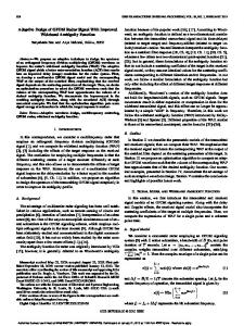
The case N = 2 is displayed in Fig. 1. As one can see, the α-part in Eq. (3) produces an attracting groove for path-oriented search strategies. If α = 1/2 the groove is V-shaped. For α < 1/2 the groove shape resembles the geometry of a black hole. Actually, it turns out that getting closer to the groove results in an increasing descent gradient towards the bottom of the groove. Its absolute value goes to infinity. That is why, it is difficult to escape from this “black groove”. Since the shape of the groove is tuneable by the α exponent, one can continuously control the problem hardness. In Fig. 2 the performance of DE, PSO, and CMA on HappyCat with N = 10 and α = 1/8 is shown. All strategies were used in a form close to their default version. DE is a Rand 3 type strategy [6], which is almost identical to the (common) DE/rand/1/bin strategy. It uses a population size of N P = 20, crossover parameter CR = 0.5, and mutation parameter F = 0.9. PSO is a local best variant with a swarm of 20 particles, parameter ϕ = 2.07 (see [7]), and 3 informants per particle. The information links between the particles are randomly chosen at the start of each iteration and a particle will always inform itself. For CMA-ES the population parameters are λ = 10 (offspring) and µ = 5 (parents). The remaining learning and cumulation

2

x2

1

0

-1

-2 -2

-1

0 x1

1

2

Fig. 1. HappyCat in two dimensions with α = 1/8 as 3D-plot (left) and contour plot (right). The latter gave rise to the funny naming of this function.

parameters are identical to the default ones used in CMA-ES version 3.55.beta obtained from URL: http://www.lri.fr/˜hansen/cmaes_inmatlab.html. p Additionally, the minimal coordinate axis deviation is set to ∀j : σ Cjj ≥ 10−7 with Cjj being an entry of the diagonal of the covariance matrix. The left plot of Fig. 2 shows the dynamics of the function value w.r.t. the number of function evaluations in a log-log format. In case of DE and PSO it represents the best function value in the current population, while for CMA it is the function value of the parent individual. The dynamics of the 3 strategies differ. CMA achieves fast progress before stagnating. PSO initially is comparable to CMA but enters the stagnation phase earlier. In contrast to CMA, the particles are able to find a region of improved fitness in later iterations (without restarting). On the other hand, DE shows a step-like characteristic where phases of stagnation are followed by small “improvement jumps”. Overall, DE is slower compared with CMA and PSO. Inspecting the final state of the population in DE and PSO reveals that they are not converged (for N = 10). For PSO, the mean distance between the particles is slightly reduced compared to the initial mean distance and a similar observation is made for the particles’ velocities. This indicates that there is “kinetic energy” left in the swarm, however, it is difficult to find improved solutions. Considering the positions of the personal best solutions, one finds that PSO tracks the groove very quickly. From that point on, progress can be made by either reducing the distance to the groove bottom or by moving toward the optimizer. Since reducing the distance to the groove bottom is much more rewarding, the personal best positions will not converge toward a single point but rather be distributed along the groove bottom. This in turn prevents a reduction in the velocities (except for the global best point) and impairs the local search behavior. For DE the situation is somewhat different. In small dimensions N ≤ 5 convergence in the experiments performed (N P = 20) is observed. There the expected population variance [8] is less than 10−14 , however, DE converges to non-optimal points. For larger search space dimensionalities, the diversity in the population remains large and similar to PSO, the points are distributed along the groove. Since DE employs a greedy selection scheme, new population members are

8

10 0

10

6

ERT/N

Function Value

10

−1

10

4

10

CMA

CMA DE

DE

2

10

PSO

PSO −2

10

Ray−ES

Ray−ES 2

10

0

3

4

10 10 Function Evaluations

5

10

10 0 10

−1

10

−2

10 Function Value

−3

10

Fig. 2. Dynamic behavior of different strategies on the HappyCat function with N = 10 and α = 1/8. In the left figure single run dynamics are shown, while in the right one the curves are based on 30 samples for each strategy. The term ERT refers to expected running time, expressed in number of function evaluations. The horizontal line in the right plot indicates the budget of function evaluations for each sample. Note, the vertical axis is normalized by the search space dimensionality N and the horizontal axis is reversed in direction. As for the fourth strategy, the Ray-ES, see Section 3.

only accepted if the distance to the groove bottom and/or the distance to the optimizer is reduced. However, the newly created individuals depend on the distances between the population members, hence only slow progress is made. In CMA, the mutation step generated by σN (0, C), with C as covariance matrix, decreases quickly. Once the mutation step is too small, the progress of CMA stops. The performance of CMA can be improved by using larger population sizes than the default one. While being slower in the early iterations a larger population size comes closer to the optimizer and has a better performance at some point. For DE and PSO no such improvement with regard to the population size is observed. Considering more than just a single run, yields the right-hand plot in Fig. 2. For all experimental runs, the necessary individual(s) for each strategy are initialized by uniformly drawing a vector from the range [−2, 2]N . The budget is set to 105 N function evaluations and 30 samples are performed for each strategy. Restarts of the strategies are allowed as long as the budget is not exhausted. In the plot the expected running time (ERT) [9] is shown as function of the best-so-far function value of all evaluated points. ERT represents the expected behavior in terms of solution quality and necessary budget. The horizontal dashed line indicates the available function evaluation budget. Points above this line indicate function values which were not achieved in all samples. In such a case the success probability is less than 1 and its inverse becomes a factor in the calculation of ERT. Therefore these data points are based on an extrapolation of the available experimental data. To achieve these performances (to a certain extent) one must increase the function evaluation budget and provide better restart criteria. Considering the trend of the ERT-curves, one observes for PSO and DE that each curves could be approximated by a straight line. This indicates a power law relation between function value and function evaluation budget. For CMA there exists a jump in the curve indi-

cating (probably) the phase where the covariance matrix is adapted. Before and after this jump a power law relation approximates the relation between function value and number of function evaluation. However, the best curve is the one for Ray-ES. This strategy can achieve an order of magnitude better solution quality (see also the left-hand plot) and is competitive with CMA and PSO in terms of function evaluations for f ≤ 10−1 . In the next section we will describe Ray-ES.

3 Ray-ES In the following we propose a concept for treating the HappyCat function. Note, this is a conceptual algorithm and not a fully developed strategy. Starting from a fixed point in the domain the idea is to find the ray direction which contains the optimizer. To this end, the strategy evolves ray directions and performs (simple) line searches along these rays to evaluate their quality. The ray evolution itself is based on the blueprint of a (µ/µl , λ)-σSA-ES [10], hence the name Ray-ES. Algorithm 1 Ray - ES 1: repeat 2: for l ← 1 to λ do 3: σ ˜l ← σeτ N (0,1) 4: y˜l ← y + σ ˜l N (0, I) y˜l 5: rl ← ky˜l k ˜ l f˜l ] ← LineSearch (rl ) 6: [x 7: end for ˜ 8: y ← hyi 9: σ ← h˜ σi 10: until termination criterion satisfied

⊲ new ray direction ⊲ new mutation strength

In Alg. 1 the pseudocode for the basic version of Ray-ES is shown. Due to the underlying design principles, one must specify values for the population sizes λ and µ, and the learning parameter τ . The parental mutation strength σ and the parental ray y ∈ RN must be initialized. From line 2 to line 7 in Alg. 1 λ new rays are created by mutation (line 4) and evaluated (line 6). The mutation operator follows the selfadaptation scheme [10], i.e. each ray has its own mutation strength σ ˜l which itself is a mutant of the parental σ (line 3). Since one is only interested in the direction of the ray, it is normalized (line 5) before being evaluated. The evaluation is performed by the ˜ l and its function LineSearch which is given in Alg. 2. It returns the best point found x corresponding function value f˜l which serves as measures for the ray quality. In lines 8 and 9 the variables for the parental mutation strength and parental ray are updated by means of intermediate recombination where the µ best of the λ offspring are used. The rule is 1 Pµ xm;λ , (4) hxi = µ m=1

where xm;λ is the mth best of the λ values. The ranking is done for all parameters w.r.t. the function value. If no termination criterion is satisfied the evolutionary process continues. Typical termination criteria are based on solution quality, budget of function evaluations, and/or measures for the stagnation of the evolutionary process.

Algorithm 2 LineSearch 1: function L INE S EARCH(r) 2: set L, k, o, ǫ 3: x0 ← o 4: ∆r ← L k 5: while ∆r > ǫ do 6: for p ← 1 to 2k + 1 do 7: xp ← x0 + ∆r(p − k − 1)r 8: fp ← F (xp ) 9: end for( 2∆r, if (x1;2k+1 = x1 ) ∨ (x1;2k+1 = x2k+1 ) 10: ∆r ← ∆r/k, otherwise 11: x0 ← x1;2k+1 12: end while 13: return x1;2k+1 , f1;2k+1 14: end function

The evaluation of a ray is a line search for the minimizer on the ray. The procedure is stated in Alg. 2. It requires the ray direction r, an initial search length L ∈ R+ , the number of subdivisions k ∈ Z+ , the ray origin o ∈ RN , and the minimal division length ǫ ∈ R acting as precision measure. Except for the ray direction all these parameters are held globally constant. In line 4, the length ∆r of the k sections is initialized. The line search (lines 5–12) is then performed as long as ∆r is greater than ǫ. At first, k equidistant points in positive and negative ray direction from the start point x0 are created (line 7) and evaluated (line 8). The start point itself is also evaluated, resulting in 2k +1 function evaluations. The best of these points, x1;2k+1 , is set as new start point (line 11). To find a better approximation of the minimizer, the length ∆r is reduced by factor k iff x1;2k+1 is not at the ends of the ray considered. However, if the current minimum is at the ends of the ray, the section length is doubled (line 10). It can be shown that the number of function evaluations for each line search can be estimated as (provided that the strategy does not leave the initial search interval [−L, L]) FEsLS ≃

L 2k ln . ln k ǫ

(5)

In the actual implementation of Ray-ES we also memorized the best-so-far solution and evaluated the center of gravity of the points returned by LineSearch. In some situations this recombinant achieved an improved solution quality. Throughout√this text the following parameter setting is used for Ray-ES: λ = 10, µ = 3, τ = 1/ N , k = 3, L = 2, o = (0, . . . , 0)N , and ǫ = 10−8 .

The single run dynamics and the expected performance for Ray-ES are shown in Fig. 2. The single run curve is based on the best value returned by LineSearch and aforementioned recombinant. Ray-ES is initially slower than the other strategies considered and needs more function evaluations per iteration. This is due to the nearly constant line search effort given by (5).1 However, at some point it is competitive with the other strategies and later achieves a solution quality not realized by the other strategies (for the parameters considered). The steep rise of the slope at the end is due to the decrease in the success probability for the function values considered.

2

f ≤ 0.1

8

10

10 PSO outlier

6

10

CMA and PSO DE

ERT

Distance to Optimizer

0

10

−2

10

4

10

CMA Ray−ES

−4

DE

2

10

10

PSO −6 10 −100

10

Ray−ES 0

−80

10

−60

−40

−20

10 10 10 Deviation from Groove

0

10

10

2

3

5 10 20 40 Search Space Dimensionality N

80

Fig. 3. The left-hand plot shows the distribution of the best solutions found in 30 samples in terms of distance to the optimizer (−1, . . . , −1) and the deviation from the groove for N = 10. The right-hand plot shows the scaling of the expected running time (ERT(f ≤ 10−1 )) for the strategies as function of the search space dimensionality N . The dashed lines represent linear and quadratic scaling, the small markers indicate the best and worst observed number of function evaluations.

In Fig. 3 additional performance plots are shown for all strategies. In the left-hand plot the distribution of the best point found in each of the 30 samples (N = 10) is shown. While PSO and CMA-ES are located at the groove bottom (horizontal axis in Fig. 3 left)2 , Ray-ES is able to achieve a much smaller distance to the optimizer (see vertical axis, there is a factor of about 10−4 ) while still being considerably close to the groove bottom. That is, the final solutions obtained by CMA, DE, and PSO are rather poor when evaluated in the search space (i.e., w.r.t. distance to the optimizer). In the right-hand plot of Fig. 3 the scaling of ERT w.r.t. the search space dimensionality is presented. The curves represent the expected running time to find a point with f ≤ 10−1 for the first time. Ray-ES shows a scaling behavior between linear and quadratic, while the other strategies have a greater than quadratic scaling behavior. In Fig. 4 the performance of Ray-ES (left) and CMA-ES (right) for various problem hardnesses is shown. In case of Ray-ES, the curve with α = 0.1 is an outlier which is 1

2

One may think of an adaptive line search to reduce FEsLS in the initial phase, however, this is beyond the scope of this paper. For visualization reasons 10−99 was added to the distance from the groove bottom.

Ray−ES

8

10

6

6

10 ERT/N

ERT/N

10

4

10

α = 0.1 α = 0.2 α = 0.3 α = 0.4 α = 0.5

2

10

0

10 0 10

CMA−ES

8

10

−1

10

−2

10 Function Value

4

10

α = 0.1 α = 0.2 α = 0.3 α = 0.4 α = 0.5

2

10

0

−3

10

10 0 10

−1

10

−2

10 Function Value

−3

10

Fig. 4. Scaling of ERT with respect to the problem hardness α for N = 10 and the default parameter settings.

due the choice of the minimal division length ǫ. Decreasing ǫ improves the performance. For CMA-ES the performances are not in order with α, i.e. α = 0.1 is easier than α = 0.2. Investigations into this behavior showed that it might be due to the frequency of restarts triggered. For small α values much more restarts occurred than for larger values. Note, we did not use stagnation as a possible restart criterion. For DE and PSO the performance improves with increasing values of α (decreasing problem hardness).

4 Conclusions and Outlook In this paper, we have proposed a new scalable test function for EAs in real-coded search spaces that allows for a continuous tuning of the problem hardness via α in Eq. (3). We have shown empirically that standard state-of-the-art EAs such as CMA-ES, DE, and PSO do fail on such topologies even in the case of small search space dimensionalities if α is chosen below a certain critical value. We also provided a proof of concept for a new class of evolution strategies, the Ray-ES, that might cope with this kind of function topologies. However, the investigations concerning this new strategy type are still in the beginning and the performance of the strategy depends on the choice of the ray origin. Yet it is a new strategy that might be worth further investigations in the future. The main purpose of this paper is test function design. From this aspect, the design principle behind HappyCat can also be used to construct more complex functions. “Complex” is meant here in the sense that the path defined by the groove can assume more complex forms than the spherical one. As an example, HGBat shall be mentioned here    2  α PN PN fHGB (x) := kxk4 − ( i=1 xi )2 + N1 21 kxk2 + i=1 xi + 21 . (6) Comparing with HappyCat (3), one sees that the quadratic symmetry-breaking part defined in (2) remains the same. The only difference is due to the first term where the expression in the bracket is a degree 8 polynomial instead of a degree 4 polynomial in

1.5 1.0

x2

0.5 0.0 -0.5 -1.0 -1.5 -1.5 -1.0 -0.5 0.0 x1

0.5

1.0

1.5

Fig. 5. HGBat in two dimensions with α = 1/4 as 3D-plot (left) and contour plot (right). The latter gave rise to the funny naming of this function resembling the silhouette of Batman’s head.

Eq. (3). The 2D shape of (6) is shown in Fig. 5. Investigations concerning this function and even more complex forms remain to be done in the future. Furthermore, it is our hope that this kind of test functions, modeling certain aspects of search and (co-) variance adaptation in constrained optimization problems, will be incorporated in the commonly used testbeds of black box optimization [9]. Acknowledgments. This work was supported by the Austrian Science Fund (FWF) under grant P22649-N23.

References [1] R. Mallipeddi and P.N. Suganthan. Problem Definitions and Evaluation Criteria for the CEC 2010 Competition on Constrained Real-Parameter Optimization. Technical report, Nanyang Technological University, 2010. [2] N. Hansen, S.D. M¨uller, and P. Koumoutsakos. Reducing the Time Complexity of the Derandomized Evolution Strategy with Covariance Matrix Adaptation (CMA-ES). Evolutionary Computation, 11(1):1–18, 2003. [3] D.V. Arnold. Analysis of a Repair Mechanism for the (1, λ)-ES Applied to a simple constrained problem. In J. Krasnogor et al., editor, GECCO-2011: Proceedings of the Genetic and Evolutionary Computation Conference, pages 853–860, New York, 2011. ACM. [4] N. Hansen and A. Ostermeier. Completely Derandomized Self-Adaptation in Evolution Strategies. Evolutionary Computation, 9(2):159–195, 2001. [5] A. I. Oyman. Convergence Behavior of Evolution Strategies on Ridge Functions. Ph.D. Thesis, University of Dortmund, Department of Computer Science, 1999. [6] Vitaliy Feoktistov. Differential Evolution: In Search of Solutions. Springer Optimization and Its Applications. Springer-Verlag New York, Inc., Secaucus, NJ, USA, 2006. [7] Maurice Clerc. Particle Swarm Optimization. ISTE Ltd., London, UK, 2006. [8] H.-G. Beyer and K. Deb. On Self-Adaptive Features in Real-Parameter Evolutionary Algorithms. IEEE Transactions on Evolutionary Computation, 5(3):250–270, 2001. [9] N. Hansen, A. Auger, S. Finck, and R. Ros. Real-parameter black-box optimization benchmarking 2010: Experimental setup. Technical Report RR-7215, INRIA, 2010. [10] H.-G. Beyer and H.-P. Schwefel. Evolution Strategies: A Comprehensive Introduction. Natural Computing, 1(1):3–52, 2002.