Hardware/Software Interface for Multi-Dimensional Processor Arrays

Hardware/Software Interface for Multi-Dimensional Processor Arrays Alain Darte CNRS, LIP, ENS-Lyon 46, Allée d’Italie 69364 Lyon Cedex 07 France [email protected]

Steven Derrien IFSIC, IRISA Campus de Beaulieu 35042 Rennes Cedex [email protected]

Abstract On most recent systems on chip, the performance bottleneck is the on-chip communication medium, bus or network. Multimedia applications require a large communication bandwidth between the processor and graphic hardware accelerators, hence an efficient communication scheme using burst mode is mandatory. In the context of data-flow hardware accelerators, we approach this problem as a classical resource-constrained problem. We explain how to use recent optimization techniques so as to define a conflictfree schedule of input/output for multi-dimensional processor arrays (e.g., 2D grids). This schedule is static and allows us to perform further optimizations such as grouping successive data in packets to operate in burst mode. We also present an effective VHDL implementation on FPGA and compare our approach to a run-time congestion resolution showing important gains in hardware area.

1 Introduction With the widespread development of systems on a chip (SoC), VLSI designers benefit from a lot of flexibility in the choice of their architectures. The conjunction of this huge design space with more and more aggressive time-to-market constraints is now a convincing argument to include highlevel design tools in SoC design methodologies. When a designer integrates a dedicated hardware accelerator in a SoC, he/she must implement an input/output protocol, composed of software and hardware parts. The software part is usually called the driver, the hardware part the interface. While the high-level synthesis research community has focused on trying to derive efficient dedicated hardware accelerators from high-level specifications, the problem of generating automatically an interface between these accelerators and the rest of the SoC has received only little attention. However, as most designers can tell, such an interface is often the most tedious and error-prone part of a

Tanguy Risset Inria, LIP, ENS-Lyon 46, Allée d’Italie 69364 Lyon Cedex 07 France [email protected]

design and it has often a strong influence on the actual performance benefits provided by the hardware acceleration. This problem is even strengthened for stream processing applications: huge parallelism is present but can be ruined by an inefficient handling of data-stream communications. We are interested in a particular class of hardware accelerators, namely regular processor arrays. Processor arrays are inherited from systolic arrays and can be automatically derived through a well-understood design methodology [11]. Pure systolic architectures happen to be impractical since they exhibit too much parallelism to meet the bandwidth and resource constraints. Strategies were proposed to derive processor arrays in the presence of resource or I/O constraints [20, 15, 12, 5, 4, 6], leading to a deep understanding of the partitioning transformation [21, 9, 6, 8]. Partitioning amounts to finding resource-constrained schedule and allocation for arbitrary large regular computations. For the design of the Pico tool [19], Darte, Schreiber, Rau, and Vivien [6] proposed an elegant theory to select a valid schedule for partitioned processor arrays, associated with an efficient implementation scheme to control the resulting architecture. Derrien and Rajopadhye [8] proposed a modeling of the partitioning problem that helps the designer choose the suitable partitioning parameters to obtain an architecture compliant with user-defined constraints. So far, none of these works address the following crucial issue: how to efficiently interface the resulting architectures to a bus. The problem of efficient interface generation of hardware IP (intellectual property) was studied in the case of linear processor arrays [16, 17, 7, 10], leading to the design of a generic master or slave interface that can be parameterized to connect to different IPs provided that they correspond to processor arrays where data is entering the array from a single processor element. Our problem has been tackled in the Paro project [2] and the Pico tool [19]. We will compare these approaches to ours in Section 4. Many interesting applications lead to multi-dimensional arrays structures such as image processing, which often makes use of 2-dimensional processors arrays. Interfacing

multi-dimensional arrays is more complicated than 1D arrays because possibly many data can enter the array simultaneously. At some point, these data have to be sequentialized in a FIFO-like channel that can be connected to a memory through a bus or a network on chip with reduced scalability. By carefully choosing the partitioning parameters, the designer can adapt on average the bandwidth required by the processor array to the bandwidth available on the communication medium [8]. But there is no guarantee that two processors of the array will not access the bus simultaneously. A natural solution is to implement a dynamic resolution of the conflicting accesses with an arbitration mechanism, as suggested in [19]. We try to promote an alternative solution by showing that a static schedule without conflict can be found for I/O of partitioned array processors. Thanks to this property, the hardware area can be reduced and, moreover, burst mode communication can further be implemented because the I/O schedule is known in advance. In this paper, we explain how to find this static I/O scheduling using the result presented in [6]. We explain our solution in the partitioning framework developed in [8]. We briefly show how the result can be generalized to ndimensional arrays. We also propose practical issues for hardware implementing the resulting arrays. We experiment this new methodology by a VHDL implementation of a partitioned matrix-product array and compare this interface mechanism to a dynamic one, showing significant improvement in the area of the resulting hardware. Further experiments are currently on-going to measure the impact of grouping communications in burst.

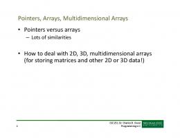
Figure 1. The SoC generic interface model. Communications between the interface and the processor array are performed with one FIFO per stream. A stream is for instance the successive pixels of an image. The term FIFO is used to model the fact that we allow a bandwidth of one data per clock cycle for each stream between the interface and the processor array, but these internal communications can be buffered in a FIFO. The hardware IP itself is a partitioned processor array obtained by the systolic design methodology. It is a 2D rectangle array of processors, which we call physical processors. Our work can be extended to n-dimensional arrays but there is probably few practical applications for such cases. These physical processors are obtained by clustering together several processors of an array of virtual processors. This clustering technique is detailed in Section 3, we briefly recall here how the virtual processor array is obtained from a high-level specification. The code below represents a matrix-matrix product expressed in the recurrence equation formalism [13]. It is usually obtained after analysis from nested loops (C or Matlab): ½ a[i, j, k]

=

b[i, j, k]

=

tmp[i, j, k]

=

c[i, j, k]

=

½

2 Target Architectural model Interface protocols and communication behavior are very dependent on architecture characteristics, thus providing a universal solution for interface is impossible. Here we state our assumptions concerning the SoC platform and the hardware accelerator, under which our result can be reused. Our target SoC is at least composed of a processor, a memory, a communication medium (bus or NoC) and a hardware accelerator (Fig. 1). The hardware accelerator is composed of a processor array that will be described later and a bus master interface. Being a bus master, the interface can initiate burst-oriented data transfers from or to the main memory. We believe that, in the context of stream processing, the use of a slave interface is very unlikely to provide enough bandwidth to our IPs. The interface shares a common clock with the processor array. Asynchronous communication with explicit handshake protocol can occur between the interface and the memory if the SoC is globally asynchronous. The interface may also contain a small amount of memory to buffer burst communications and/or a bus arbiter if a dynamic communication scheme is used.

A[i, k] a[i, j − 1, k]

if j = 0 if 0 < j < M

B[k, j] b[i − 1, j, k]

if i = 0 if 0 < i < N

a[i, j, k] ∗ b[i, j, k] ½ tmp[i, j, k] c[i, j, k − 1] + tmp[i, j, k]

if k = 0 if 0 < k < P

Using the systolic design methodology implemented for instance in MMAlpha [11], one can transform this specification by successive operations on the dependence graph (depicted in Fig. 2 for the parameter values N = M = P = 3). Each node of the graph represents one execution instance of the body of the loop. The schedule assigns an execution date to each of them. Due to the possibly large (or even parameterized) size of the graph, the scheduling is regular, expressed as a linear function of the index ~i = (i, j, k), which identifies a single operation in the algorithm. The schedule is represented on Fig. 2 with shaded hyperplanes, here as i + j + k. Finally a virtual processor array of size N × M can be designed by mapping the dependence graph to an architecture, here by a projection along the third axis, i.e., (i, j, k) is mapped onto the virtual processor (i, j). In general, the loop nest to be implemented in hardware may have more than 3 indices and each loop iteration is referenced by its index vector ~i = (i1 , . . . , in ), where n is the loop depth.

t = 2

t = 2

t = 4 t = 5 t = 6

t = 1

t = 0

~ e3 = [001] ~ e2 = [010] ~ e1 = [100]

P0,0

P0,1 P1,0

P0,2 P1,1 P2,0

P1,2 P2,1

P2,2

Figure 2. Matrix-matrix product example. It will then give rise to a (n − 1)-dimensional virtual array. For further reading on the systolic methodology, see [18]. Partitioning (a.k.a. co-partitioning) includes two parts: tiling (or LPGS partitioning) and clustering (or LSGP partitioning). Tiling cuts the virtual processor space into tiles that are processed, one after the other, by the hardware accelerator. If the on-chip memory is not large enough to store the complete set of data flowing in the array, intermediate results are stored in an off-chip memory. We do not address tiling in this paper as most of the communication work during the execution of tiles is done by the software driver. We will rather concentrate on the clustering part. Clustering an array is the action of assigning the work of a hyper-rectangle (or cluster) of virtual processors to a single physical processor. This cluster is of size σ1 × . . . σn−1 as we have (n − 1) dimensions in the virtual processor array. After clustering, we obtain a physical array, usually of dimension 2. Fig. 3 represents (on the left) a virtual array for the matrix-matrix product, for parameter values N = M = 4, and a physical array obtained by clustering with a cluster of size σ1 × σ2 = 2 × 1 (on the right). The σi parameters are chosen to adapt the bandwidth of the physical array to the bandwidth available on the SoC. For a clustering to be valid, the dates at which virtual processors are active must be distinct so that they can be sequentialized on the physical processor. In [6], this physical processor is said to juggle with the virtual computations. It is also explained how to compute such valid schedules given the respective sizes of the virtual and physical arrays envisaged. Once this schedule is computed, it is fixed, one cannot modify the internal behavior in order to change input/output dates. So far, we did not talk about input/output of the array. We suppose that the I/O of the virtual array occur on the boundary processors of the array. As shown on the left of Fig. 3, one stream (the matrix B) enters from the left in the processors with p1 = 0, one stream (the matrix A) enters from the bottom in the processors with p2 = 0, and one stream (the matrix C) is output on the right in the processors with

p1 = 3. On the right of this figure, i.e., in the corresponding physical array, we show the mechanism that we target for bringing the data from the bus to each physical processor. We associate with each stream one FIFO (connected to the bus) and one shift register. Each shift register has a certain number r of registers between successive processors. For instance, here, the shift register corresponding to A has r = 4, the shift register used for the output of the matrix C has r = 2 registers between successive physical processors. This is the model of our interface. We will show that, given a schedule of the computations that has been fixed by the clustering, we can always find values for the r such that there are no conflict at the FIFO level, i.e., two data of the same stream enter their shift register at different dates. φ

p2

σ2

p2 (0,3)

(1,3)

(2,3)

(3,3)

(0,2)

(1,2)

(2,2)

(3,2)

(0,1)

(1,1)

(2,1)

(3,1)

(0,0)

(1,0)

(2,0)

(3,0)

FIFO

FIFO

σ1

p1

FIFO

φ

p1

Figure 3. Virtual and physical processor arrays, with σ1 × σ2 = 2 × 1. The I/O feeding of the physical array is shown on the right.

3 Juggling with I/O 3.1 LSGP partitioning scheme An architecture derived with the LSGP (locally sequential globally parallel) partitioning methodology is fully defined by a schedule, an allocation, and a cluster shape: Schedule: the operation identified by the vector ~i, of dimension n, is computed at time ~τ .~i (dot product), i.e., the schedule is defined by a 1D linear function of ~i. Allocation: the operation ~i is mapped onto the virtual processor identified by the vector ~q = Π~i, of dimension (n − 1), where Π is the matrix formed by the (n − 1) first rows of a unimodular matrix Q of size n × n. Clustering: each virtual processor ~q is mapped to the physical processor ~q φ such that qkφ = b σqkk c where σk is the k-th cluster size. We let ~q c such that qkc = qk mod σk . The schedule is constrained by flow dependences and by the fact that no two virtual processors in a hyper-rectangular “box” of size σ1 × · · · × σn−1 are simultaneously active: in this case, a physical processor can indeed emulate all of them in a sequential manner (schedule with no conflict). When, in addition to this juggling constraint, each physical processor is active at each clock cycle in the steady state, the schedule is said to be tight [6].

From now on, we work with p~ = Q~i (change of basis): the operation identified by p~ is then computed at time ~τ .(Q−1 p~) – still a linear 1D function – and mapped onto the virtual processor ΠQ−1 p~ which is simply (p1 , . . . , pn−1 ). We assume the physical array is a hyper-rectangle array of size P1 × · · · × Pn−1 and that values are propagated inside the array, thanks to a routing technique [14], so that I/O take place on a face of the virtual array, i.e., correspond to all virtual processors with pk = 0 (or the opposite face), for some 1 ≤ k ≤ n−1. The problem is now to find a way to route all I/O from the FIFO, connected to the bus master interface, to the physical processors that need them, with the constraint that the FIFO can deliver at most one data per cycle. Before addressing this routing problem, let us see how an LSGP-partitioned architecture is obtained following the methodology of Derrien and Rajopadhye [8]. Starting from the architecture described by virtual processors, the schedule and allocation are changed by a sequence of elementary transformations, skew, slow down, and serialization, whose effect can be directly interpreted in the architecture representation. We illustrate this process on the face p2 = 0 (see Fig. 4) of the virtual array of Fig. 2, here with schedule t = i+j +k = p1 +p2 +p3 and allocation (p1 , p2 ) = (i, j).

× +

t

0

p1

Figure 5. Skew by −1 in direction 1 on Fig. 4. different activation dates. Fig. 7 shows a skew by 1, followed by a serialization by 3, in direction 1, for the architecture of Fig. 6. A processor emulates 3 virtual processors (identified with different patterns). The resulting hardware is modified in a systematic way: multiplexers are added for the connections that are “crushed” and are controlled with a 1-bit rotating register. Serialization does not affect the schedule but affects the allocation. With pci = pi mod σ, pφi = b pσi c, the new allocation function is (pφ1 , p2 ). In [6], it is proved that a linear schedule τ is tight for a cluster shape σ1 ×. . .×σn−1 if and only if it has the following form, up to a permutation of the processor dimensions: τ (p1 , . . . , pn−1 , pn ) = λ1 p1 + σ1 (λ2 p2 + σ2 (. . . +σn−2 (λn−1 pn−1 ± σn−1 pn ) . . .))

B2,0 B1,0 B0;0 × +

0

Ctrl

t

C2,0

p1

(1)

where λi and σi are relatively prime. This is a sequence of slow down by σi and skew by λi (for serialization of σi ) in dimension i, starting from the schedule equal to pn or, more generally, any schedule such that any virtual processor is active at each cycle. We will use this result to define a schedule for the FIFO that “juggles” with the I/O.

A2,0 A2,1 A2,2

Figure 4. Activity for p2 = 0. A skew by λ in direction i adds λ registers (or deletes |λ| if λ < 0) on each data flow path parallel to direction i. A skew by −1 in direction 1 for the architecture of Fig. 4 is given in Fig. 5 together with its consequences on the internal processor architecture. A skew changes the schedule, it “adds” λpi clock cycles. In Fig. 5, the schedule is now p2 + p3 and Ai,k (represented by p~ = (i, 0, k)) enters the array in virtual processor (p1 , p2 ) = (i, 0) at time 0 + p3 = k. A slow down by c replicates c times each register, leading to an architecture that behaves c times slower. Fig. 6 shows a slow down by 3 after the previous skew. The new schedule is 3(p2 + p3 ) and Ai,k enters the virtual array at step 3(p2 + p3 ) = 3k in processor (p1 , p2 ) = (i, 0). A serialization by σ in direction i maps σ successive virtual processors in direction i on 1 physical processor. For a serialization to be valid, the σ virtual processors must have

× +

0 t

p1

Figure 6. Slowdown by c = 3 on Fig. 5.

3.2 Valid I/O schedules We now focus on the I/O schedule at the processor array boundaries. Obviously, this schedule directly derives from the partitioned array schedule. If we look back at the peripheral interface template, Fig. 3, we see that data associated

when pφk is constant), the FIFO is connected to a sequence of (n − 2) shift registers along dimension j 6= k, each of size rj between two successive physical processors. In Fig. 3, when accessing the face pφ2 = 0 (here a line, for propagating A), there are r1 = 4 registers between successive processors on the boundary. We denote by τIk/ O the function that gives the time at which the data used in a physical processor is present at the FIFO output port, when routing for dimension k. The I/O schedule τIk/ O can be deduced from the schedule τ and from the number of registers rj , j 6= k: τIk/ O (pφ1 , . . . , pφn−1 , pc1 , . . . , pcn−1 , pn ) = τ (pφ1 , . . . , Pn−1 pφn−1 , pc1 , . . . , pcn−1 , pn ) − j=1, j6=k rj pφj

p

φ

p1 = b 31 c

p1

1 0

×

×

+

+

0

1 00

0

0 1

Figure 7. Skew by 1 and serialization by 3. to a given stream are read/written from/to a FIFO linked either to CPU or memory. All boundary processors access the same FIFO, possibly at the same time, hence causing conflicts. Finding a valid routing is not obvious even when, on average, the amount of data requested is low enough. A runtime arbitration technique can be used but would certainly degrade performance (wait states) and increase the resource usage (arbitration logic). Our goal is to find an efficient mechanism to route the input data from the FIFO output to the processor input ports (the converse for output data), and to generate the associated control circuitry. We want to do it at compile time, through a static routing schedule. We first formulate the I/O schedule for boundary processors in a partitioned array, focusing on one particular stream. Each operation identified by p~ = (p1 , . . . , pn ) is scheduled at time τ (~ p) and mapped to the virtual processor α(~ p) = (p1 , . . . , pn−1 ). After clustering, the allocation is αφ (~ p) = (pφ1 , . . . , pφn−1 ) with pk = pφk σk + pck , 0 ≤ pck < σk . It is no longer linear, except if we describe it (and the schedule) in a space of dimension (2n−1) indexed by (pφ1 , . . . , pφn−1 , pc1 , . . . , pcn−1 , pn ). Thus, when parameters σk are known, we can perform further transformations on the physical architecture, still within a linear framework. To access an array boundary in dimension k (i.e.,

(2)

If the rj are such that τIk/ O (~ p) 6= τIk/ O (~q) for all p~ 6= ~q that correspond to I/O operations, with pk = qk = 0, then τIk/ O is a valid I/O schedule for routing on the face pk = 0. Example Consider in Fig. 8, the array with 3 physical processors (grey boxes) on the pφ1 = 0 boundary, obtained thanks to a clustering 3×2, and scheduled with the schedule τ (pφ1 , pφ2 , pc1 , pc2 , p3 ) = 2pc1 + pc2 + pφ2 + 6p3 . This schedule is tight: each physical processor emulates the same virtual processor after 6 cycles (because of 6p3 ) and no two virtual processors are active at the same time (for a fixed (pφ1 , pφ2 ), the schedule is of the form given by Equ. 1). It meets the bandwidth requirement because 6 data are sent during 6 cycles (each processor needs 2 data every 6 cycles). But if we assume that data are broadcast from the FIFO to each processor, the resulting I/O schedule τI1/ O is not valid (see Fig. 8, the large circles mean that more than one data need to be sent). Now, if we assume another communication mechanism for bringing data from FIFO to processor, as in Fig. 9, i.e., with r2 = −1, the I/O schedule τI1/ O is now valid. ¤ time (0,5)

(1,5)

(2,5)

p ~ φ = (0, 2) (0,4)

(1,4)

(2,4)

(0,3)

(1,3)

(2,3)

p ~ φ = (0, 1) (0,2)

(1,2)

(2,2)

(0,1)

(1,1)

(2,1)

p ~ φ = (0, 0) (0,0) p2 FIFO output

p1

(1,0)

(2,0)

σ2 = 2

t

t

σ1 = 3

Figure 8. Conflicting I/O schedule: at time t = 1, 2, 7, 8, several processors access the FIFO (conflicts shown as large black circles).

3.3 How to get valid I/O schedules Let γ be the coefficient of pn in the schedule τQ : each virtual processor is active every |γ| cycles (|γ| ≥ j σj ,

time (0,5)

(1,5)

(2,5)

p ~ φ = (0, 2) (0,4)

(1,4)

(2,4)

(0,3)

(1,3)

(2,3)

(0,2)

(1,2)

(2,2)

(0,1)

(1,1)

(2,1)

p ~ φ = (0, 0) (0,0) p2 FIFO output

p1

(1,0)

(2,0)

σ2 = 2

p ~ φ = (0, 1)

σ1 = 3

Figure 9. The I/O schedule is dense (FIFO accessed every cycle) and conflict free (at most one access to the FIFO at a given cycle). with equality when the schedule is tight). The number of dimension k is Q physical processors on the face along Q P . Each processor emulates σ virtual procesj j j6=k j Q sors, and j6=k σj of them correspond to I/O. Thus, on average, Q the number of I/O on the face along dimension k is ( j6=k Pj σj )/γ, which should be Q less than 1. Thus, the physical array must be such that j6=k Pj ≤ Q γ σj . This j6=k Q means j6=k Pj ≤ σk when τ is tight, otherwise this last condition is stronger. We call it the strong condition. The register numbers rj must be chosen such that, in the box 0 ≤ pφj < Pj , 0 ≤ pcj < σj , j 6= k, pφk = pck = 0 (i.e., pk = 0), at most one element is active at a given cycle, according to the schedule τIk/ O , i.e., the FIFO juggles with I/O. Therefore, the problem is formulated again as a clustering problem, here in dimension 2(n − 2) and we can reuse the techniques developed in [6], in particular the characterization Q of tight schedules (Equ. 1). We now show that, when j6=k Pj ≤ σk , suitable values for the rj can be automatically derived without restriction on the dimension n − 1 of the virtual processor array. When routing for the face along dimension k = 1 (w.l.o.g), the trick is to exploit the fact that each physical processor juggles with its virtual processors indexed by (pc1 , . . . , pcn−1 ) in the box of size σ1 ×. . .×σn−1 , so as to define a schedule τI1/ O such that the FIFO juggles with all virtual processors (pφ2 , . . . , pφn−1 , pc2 , . . . , pcn−1 ) in the box of size (P2 × . . . × Pn−1 ) × (σ2 × . . . × σn−1 ). We first consider the simplest case of a 2D processor array, obtained by clustering a virtual processor array of dimension n − 1 ≥ 2. Suppose, w.l.o.g., that Pj = 1 for all j ≥ 3, and that the I/O routing needs to be done for the face pφ1 = 0, along dimension 2, i.e., only the value r2 needs to be defined. Since, for the I/O, we are interested in the computations such that p1 = 0, the I/O schedule is τI1/ O = γpn + τ2 pc2 + . . . + τn−1 pcn−1 + (α2 − r2 )pφ2 + α3 pφ3 + . . . + αn−1 pφn−1 (see Equ. 2 with p1 = 0). For j ≥ 3, Pj = 1 thus α3 pφ3 +. . .+αn−1 pφn−1 is constant and, w.l.o.g, we can work with τI1/ O = γpn + τ2 pc2 + . . . + τn−1 pcn−1 + (α2 − r2 )pφ2 . In

each cluster, the schedule τ = γpn +τ1 pc1 +. . .+τn−1 pcn−1 juggles. If P2 ≤ σ1 (strong condition), we can choose r2 such that α2 − r2 ≡ τ1 mod γ and we get a valid I/O schedule: indeed, the fact that each physical processor juggles in the box (pc1 , . . . , pcn−1 ) of size σ1 × . . . × σn−1 implies that the FIFO juggles with all I/O corresponding to the box (pφ2 , pc2 , . . . , pcn−1 ) of size (P2 ×σ2 ×. . .×σn−1 ). When Q the schedule is tight in each physical processor, i.e., γ = σj , a more accurate analysis reveals that we have more freedom to choose r2 . The coefficient τ1 in the schedule τ has the form λ1 ρ where λ1 and σ1 are relatively prime (see Equ. 1 again, here ρ is the product of some σj , j 6= 1). If we choose r2 such that α2 − r2 = λ0 ρ, where λ0 and σ1 are relatively prime, we get a schedule τI1/ O of the same form as τ , but with pφ2 instead of pc1 , thus valid for our FIFO constraints. Example (Cont’d) Consider again the example in Fig. 8, with the tight schedule 2pc1 + pc2 + pφ2 + 6p3 . For a fixed pφ2 , the schedule τ = pc2 +2pc1 +6p3 juggles for the box (pc1 , pc2 ) of size 3 × 2, with τ2 = 1 and τ1 = λρ = 1 × σ2 = 2. If we choose r2 = −1 (as in Fig. 9), α2 − r2 = 2 = λ0 ρ with λ0 and σ1 relatively prime, and we get the I/O schedule τI1/ O = pc2 + 2pφ2 + 6p3 , of same form as τ , thus valid if P2 ≤ σ1 = 3. We could also choose r2 = 3 since α2 − r2 is then 1 − 3 = −2, also of the required form. ¤ For a 3D processor array (thus with routing in 2D) things are more complicated, but still manageable. Suppose we route for the face pφ1 = 0 along dimensions 2 and 3. The difficulty is that, now, we need to play with a correspondence between a 1D space (the pc1 dimension, 0 ≤ pc1 < σ1 ) and a 2D space where the routing takes place (the dimensions (pφ2 , pφ3 ) and not only pφ2 as before). If P2 P3 ≤ σ1 , we can apply a similar trick. We first “linearize” conceptually the indices that describe the 2D box of size P2 × P3 into an index in a 1D box of size P2 P3 (smaller than σ1 with the strong condition), for example (pφ2 , pφ3 ) → pφ2 +P2 pφ3 . Then, we apply the same techniques as before. The first one leads to r2 and r3 such that, for all pφ2 , pφ3 , (α2 −r2 )pφ2 +(α3 −r3 )pφ3 ≡ τ1 (pφ2 +P2 pφ3 ) mod γ, i.e., α2 − r2 ≡ τ1 mod γ and α3 − r3 = τ1 P2 mod γ. The second technique leads to r2 and r3 such that (α2 − r2 )pφ2 + (α3 − r3 )pφ3 ≡ λ0 ρ(β2 pφ2 + β3 pφ3 ) where λ0 and ρ are as before, and β2 pφ2 + β3 pφ3 mod σ1 juggles in the box P1 × P2 . The situation is the same in higher dimensions. The resulting shift registers are more likely to be larger than the number of live values they contain, thus alternative hardware support such as shift queues [1] could be useful.

4 Efficient hardware synthesis To illustrate the benefits of our approach, we compare our interface implementation to an alternative one based on a run-time management of the I/O conflicts. In this case,

whenever two or more processors have to perform an I/O for the same stream at the same time, a hardware arbiter is used to select which access will be scheduled first. In this alternative approach, processors have a direct access to the I/O bus, and they must be able to compute the addresses from (resp. to) which they need to read (resp. write). For that, each processor must integrate a local controller to compute the current iteration coordinates, determine whether this iteration requires an I/O, and further retrieve the I/O address from the iteration coordinates. Our local controller implementation follows the approach of [6]. A simple hardware arbiter sequentializes simultaneous I/O requests (run-time conflicts) with a simple fixed-priority encoder. To get a reasonable clock-period, we put a register between the arbiter and each physical processor, for each stream. This run-time arbitration design is very likely to induce an area overhead: the local control within processors is more complex than in our approach (in which both I/O and local control are handled through simple shift-register hardware structures). Besides, this run-time management does not scale well, as the arbiter complexity and the number of multiplexers grow linearly with the number of processors, and directly impacts the interface critical path. We prototyped (in VHDL) the two approaches for the matrix-matrix product (note that the choice of this basic example does not affect the validity of the results, as any 2D processor array will use a similar interface1 ). This VHDL description is designed to offer a maximum of flexibility: several parameters of the architecture can be configured (physical array size, partitioning parameters, etc.). The code was written by hand, following the theory explained in previous sections; we are working on the automation of this process in MMAlpha. For both approaches, we synthesized a set of architecture instances that only differ by some parameters for which we gathered experimental results in terms of estimated resource usage (estimated maximum operating frequency are similar in both cases and thus not given). The synthesis was done using Synplify. A summary of the results is given in Table 1; to make a fair comparison, one should compare the sum of LUT and SRL16 (for the static interface) to the number of LUT in the run-time approach, and the DFF for both approaches. Experiments show that our approach based on a static I/O schedule leads to significant area savings: while the number of flip-flops (DFF) required to implement the interface is roughly the same in both approaches, the number of LUT resources is much lower in our approach especially for larger processor arrays. The selected values for the rj parameters depend on the scheduling functions, which are not detailed here. We point out that the values of the rj barely affect the area cost of the interface. This is due to the use of the Xilinx shift-register primitives, which can pack shift-registers, up 1 Things

are slightly more complicated for 3D arrays, see Section 3.3.

Matrix N × N × N and physical array shape N shape 32 2×2 32 4×4 32 8×4 64 4×4 64 8×4 64 4×8 64 8×8 128 8×8 128 8×4 128 16 × 4 128 16 × 8

Area static LUT / DFF / SRL 16 116 96 128 116 96 256 116 96 320 132 102 256 132 102 320 132 102 448 132 102 512 156 108 512 156 108 320 156 108 448 156 108 640

run-time LUT / DFF

285 539 698 603 784 1048 1217 1454 970 1343 1811

266 508 640 532 672 888 1064 1160 768 1096 1472

Table 1. Experimental results for interface area: number of logic cells (LUT), of registers (DFF), and of Xilinx shift registers primitives (SRL16) (not used in the run-time approach). to 16-bit deep, into a single logic cell. Besides, these area improvements are not the only benefits: we don’t suffer from the performance penalty due to the arbitration wait states during an I/O conflict, and we know statically the order in which I/O are performed. This latter property is very important in practice. Indeed, we mentioned in Section 2 that our interface should be packet-oriented: to obtain reasonable I/O performance from the bus protocol, our interface should be able to perform grouped I/O, i.e., accesses to several contiguous memory words, in burst mode. But, for a given stream, the sequence of I/O on the FIFO very seldom accesses contiguous memory words (actually, this is more like an exception), it is thus not possible to directly benefit from grouped I/O (note that this problem is similar in the case of the run-time arbitration interface). However, unlike the run-time approach, since our interface is based on a static schedule of I/O operations, we know in advance the order in which memory words should be accessed. We can thus use a reordering memory, which acts as a buffer between the routing shiftregisters and the bus interface (this line buffer is sketched in Fig. 1). This allows the bus master controller to write (resp. fetch) packets of contiguous words to (resp. from) memory, while on the processor array side, our routing mechanism will access this memory using its own address sequence. We believe that this reordering memory is likely to play an important part in the effective performance of our interface; our ongoing work focuses on finding a suitable control and synchronization mechanism to handle this buffer, and how to determine a minimum upper bound for its size. As mentioned in the introduction, a similar problem was studied in [2, 19]. The work of [19] is more advanced since it gave rise to the commercial tool Pico, but their arbitration mechanism is only sketched. The comparison with our strategy given in this section shows that a static schedule can

provide improvements. The problem addressed by Bednara and Teich is similar to ours, but their target processor array and interface protocol are different: they target a slave IP and their handling of resource constraints is not based on juggling. As far as we could understand their papers [2, 3], they allow software pipelining in the processors (we do not), but they don’t take into account idle cycles in boundary processors (as in our case, Fig. 8). This results in a repetitive schedule which acts as if an I/O needs to be done in each initiation interval. Thanks to our juggling modeling, we can take into account cycles where no communication occurs and only schedule real communications. Another advantage is that we can reuse the control mechanisms (address generation and activity control) used in the Pico tool, which is well documented, while the controllers of [2] are not detailed. We also have experimental results concerning the resulting VHDL, which will be interesting to compare with Bednara and Teich results if some are provided in the future.

5. Conclusion We have extended the LSGP partitioning theory to take into account I/O constraints and automatically generate an efficient hardware/software interface for hardware accelerators in a SoC. Rather that proposing a new formulation, we use the resource-constrained “juggling” technique developed in [6] to schedule the I/O of a processor array so that no collisions occur on the on-chip communication medium. Our first VHDL hardware implementation shows that the complexity of the resulting mechanism is better than with previous approaches. We hope to show further improvements in the latency of the communication using the burst mode. We are currently studying the possibility of implementing the method in MMAlpha.

References [1] S. Aditya and M. S. Schlansker. ShiftQ: A buffered interconnect for custom loop accelerators. In International Conference on Compilers, Architecture, and Synthesis for Embedded Systems (CASES’01), pages 158–167, Atlanta, USA, 2001. ACM Press. [2] M. Bednara and J. Teich. Interface synthesis for FPGAbased VLSI processor arrays. In International Conference on Engineering of Reconfigurable Systems and Algorithms (ERSA-02), Las Vegas, Nevada, U.S.A., 2002. [3] M. Bednara and J. Teich. Automatic synthesis of FPGA processor arrays from loop algorithms. Journal of Supercomputing, 26:149–165, 2003. [4] A. Darte. Regular partitioning for synthesizing fixed-size systolic arrays. Integration, The VLSI Journal, 12:293–304, Dec. 1991. [5] A. Darte and J.-M. Delosme. Partitioning for array processors. Technical Report 90-23, LIP, École normale supérieure de Lyon, France, 1991.

[6] A. Darte, R. Schreiber, B. R. Rau, and F. Vivien. Constructing and exploiting linear schedules with prescribed parallelism. ACM Transactions on Design Automation of Electronic Systems, 7(1):159–172, 2002. [7] S. Derrien, A.-C. Guillou, P. Quinton, T. Risset, and C. Wagner. Automatic synthesis of efficient interfaces for compiled regular architectures. In International Samos Workshop on Systems, Architectures, Modeling, and Simulation (SAMOS’02), Samos, Greece, July 2002. [8] S. Derrien and S. Rajopadhye. Loop tiling for reconfigurable accelerators. In 11th International Symposium on Field Programmable Logic (FPL’01), 2001. [9] D. Fimmel. Generation of scheduling functions supporting LSGP-partitioning. In IEEE International Conference on Application-specific Systems, Architectures and Processors (ASAP’00), pages 349–358, Boston, July 2000. [10] A. Fraboulet and T. Risset. Efficient on-chip communications for data-flow IPs. In IEEE International Conference on Application-specific Systems, Architectures and Processors (ASAP’04), pages 293–303, 2004. [11] A.-C. Guillou, P. Quinton, T. Risset, C. Wagner, and D. Massicotte. High-level design of digital filters in mobile communications. DATE Design Contest 2001, 2nd place, Mar. 2001. Available as IRISA Research Report 1405. [12] F. Irigoin and R. Triolet. Supernode partitioning. In 15th Annual ACM Symposium on Principles of Programming Languages, pages 319–329, San Diego, CA, Jan. 1988. [13] R. M. Karp, R. E. Miller, and S. Winograd. The organization of computations for uniform recurrence equations. Journal of the ACM, 14(3):563–590, July 1967. [14] M. Manjunathaiah, G. M. Megson, T. Risset, and S. Rajopadhye. Uniformization of affine dependence programs for parallel embedded system design. In L. M. Ni and M. Valero, editors, International Conference on Parallel Processing (ICPP’01), pages 205–213, 2001. [15] D. Moldovan and J. A. B. Fortes. Partitioning and mapping algorithms into fixed-size systolic arrays. IEEE Transactions on Computers, 35(1):1–12, jan 1986. [16] J. Park and P. C. Diniz. Synthesis of pipelined memory access controllers for streamed data applications on FPGAbased computing engines. In International Symposium on System Synthesis (ISSS’01), pages 221–226, 2001. [17] J. Park and P. C. Diniz. Synthesis and estimation of memory interfaces for FPGA-based reconfigurable computing engines. In International Symposium on FPGA Custom Computing Machines, 2003. [18] P. Quinton and Y. Robert. Systolic Algorithms and Architectures. Prentice Hall and Masson, 1989. [19] R. Schreiber, S. Aditya, B. R. Rau, V. Kathail, S. Mahlke, S. Abraham, and G. Snider. High-level synthesis of non programmable hardware accelerators. In IEEE Int. Conference on Application-specific Systems, Architectures and Processors (ASAP’00), pages 113–126, Boston, July 2000. [20] W. Shang and J. A. B. Fortes. Independent partitioning of algorithms with uniform dependencies. In Int. Conference on Parallel Processing (ICPP’88), pages 26–33, 1988. [21] J. Teich, L. Thiele, and L. Zhang. Partitioning processor arrays under resource constraints. International Journal of VLSI Signal Processing, 17(1):5–20, 1997.