harmonic load identification based on fast fourier transform and ...

Journal of Theoretical and Applied Information Technology 15th March 2017. Vol.95. No 5 © 2005 – ongoing JATIT & LLS

ISSN: 1992-8645

www.jatit.org

E-ISSN: 1817-3195

HARMONIC LOAD IDENTIFICATION BASED ON FAST FOURIER TRANSFORM AND LEVENBERG MARQUARDT BACKPROPAGATION 1

INDHANA SUDIHARTO, 2 DIMAS OKKY ANGGRIAWAN, 3 ANANG TJAHJONO 1 Assoc. Prof., Department of Electrical Engineering, Politeknik Elektronika Negeri Surabaya, Indonesia 2

Instructor, Department of Electrical Engineering, Politeknik Elektronika Negeri Surabaya, Indonesia

3

Assoc. Prof., Department of Electrical Engineering, Politeknik Elektronika Negeri Surabaya, Indonesia E-mail: [email protected], [email protected], [email protected]

ABSTRACT One of the most important power quality problems in power system is harmonic distortion. Due to an increase of non-linear loads as harmonic sources, the identification of harmonic loads becomes important concern in the power system. Therefore, this paper proposes a Levenberg Marquardt Backpropagation (LMBP) Neural Network to identification of harmonic load. Data of harmonic load are gathered from a low cost microcontroller with Fast Fourier Transform (FFT) method as analysis of the input current waveform in the presence of multiple devices to obtain the harmonic value. LMBP is trained using harmonic as input with combination of 14 different types of load. The performance of LMBP is implemented with several of the different training and test data to validate the accuracy and efficiency of the proposed algorithm. The results show that the proposed algorithm has high accuracy to determine the presence of loads based on their harmonic signature. Keywords: Levenberg-Marquardt Backpropagation (LMBP), Harmonic, Fast Fourier Transform (FFT), load identification, low cost microcontroller 1.

important role in keeping a level of harmonic distortion in consistent with the standard [3].

INTRODUCTION

Now days, the increasing of non-linear load such as computers, LHE lamps, monitors, variable speed drives, UPS and other electronic devices become an important issue in the power system. One of the very important issue caused by the presence of these devices are harmonic distortion. Harmonic could produce power quality problems such as voltage distortion, equipment malfunction, poor quality of power factor and component failure. Moreover, harmonic distortion also causes financial loss of the customers and electric power companies [1]. Harmonic sources is required to identify various types of devices. With this identification, power system operators can decide a strategy to reduce harmonic distortion level with filter placement [2]. Refers to IEEE Standard 519-1992 (IEEE Recommended Practices and Requirements for Harmonic Control in Electrical Power Systems) sets limits for acceptable levels in the harmonic current in the power system. Therefore, costumer plays an

Techniques to harmonic source detection in [4] and [5], presented state estimation technique with least square estimation to identified the harmonic source. H. Ma et al [5], presented kalman filter technique to identification of harmonic source. Technique to identify residential loads, the current waveform in [6] and [7] are used, where monitoring residential loads using appliance signatures. Robertson et al, [8] used wavelet transform for load identification with unknown transient behaviors. However, this technique is expensive because to detect the transient behavior, powerful devices is required. Cole et al, [9], [10] load identification algorithm uses load switching between individual appliances. But, this algorithm cannot be recognized if any appliance does not change. Therefore, load identification uses harmonic is proposed in this paper to mitigate the disadvantages of the previous published research. Classification capabilities of artificial neural network are used in power quality studies, fault and

1080

Journal of Theoretical and Applied Information Technology 15th March 2017. Vol.95. No 5 © 2005 – ongoing JATIT & LLS

ISSN: 1992-8645

www.jatit.org

harmonic source classification [11], [12]. Harmonic components are evaluated as sources of valuable information for load identification. Levenberg Marquardt Backpropagation (LMBP) is developed for load identification [13], [14], [15], [16]. This model is trained using harmonic component data. Fast Fourier Transform (FFT) as analysis of the input current waveform in the presence of multiple devices. This model can identify the devices from the current harmonics. LMBP is trained using harmonic data with combination of 14 different types of load. The performance of LMBP is implemented with several different training and test data to validate the accuracy and efficiency of the proposed algorithm. The results for harmonic load identification using LMBP with 10 neurons have very minimal average percentage error of 0.11%.

THD value. It could be concluded that each data contain 9 attributes. Each combination taken 100 samples of data so there are 1400 samples data that will be used in this experiment. These data will be divided into training data and test data for training and testing 2.2. Input of LMBP A low cost microcontroller STM32F407VGT66 can measure the harmonic data at 1, 3, 5, 7, 9, 11, 15 and Total Harmonics Distortion (THD). Therefore, there will be 9 attributes and 14 classes. Identification on LMBP is done by determining the pattern of the combination of non-linear loads connected as input data for the training phase and testing phase. These four non-linear loads are ranged in 14 combinations of loads as follows Table 1. Non-linear load combinations

The main contribution of this paper is harmonic data from non-linear loads are gathered and analyzed with FFT using low cost microcontroller in real time mode and harmonic used as input LMBP for load identification. The organization in this paper is as follows. In section 2, Introduction load identification system is described. In section 3, Hardware component is presented. In section 4, LMBP is discussed. In section 5, the analysis of the simulation result. In section 6, conclusion of this paper is described. 2.

LOAD IDENTIFICATION SYSTEM

2.1. Data Capture Firstly, the study is begun with collecting harmonic currents and THD data. The data is obtained through the measurement of four different types of non-linear loads based on a low cost microcontroller with FFT analysis which is a research laboratory B204 in the range 0-5 A. Four types of non-linear load used in this measurement process consists of SHARP AC, Simbadda S – 2660 PC, ACER 4755G portable computer, and two 23 Watt energy saving lamps Philips. These non - linear loads are ranged into 14 combinations and each combination of data taken from the first up to - 15 harmonics as well as THD data. Once the load combinations specified, then the measurements were taken using a low cost microcontroller with FFT analysis. Measurement result of the load combination are the currents, only the odd-numbered harmonics from the fundamental to the 15th harmonic and the

E-ISSN: 1817-3195

3.

Combination

AC

PC

Laptop

Lamp

1

0

0

0

1

2

0

0

1

0

3

0

0

1

1

4

0

1

0

0

5

0

1

0

1

6

0

1

1

0

7

0

1

1

1

8

1

0

0

0

9

1

0

0

1

10

1

0

1

0

11

1

0

1

1

12

1

1

0

0

13

1

1

0

1

14

1

1

1

0

HARDWARE COMPONENTS

The implementation of hardware is described in this section. Harmonic and power components computation is applied in the hardware consists of ARM microcontroller STM32F407VGT6 as processor device for computation, ACS712 as current sensor, AMC1100 as voltage sensor and LCD-32PTU as display device. ARM microcontroller STM32F407VGT6 is selected for implement harmonic and power components computation because it is a high performance microcontroller. This microcontroller operates 167 MHz that provides high performance for signal processing that requires high accuracy and speed.

1081

Journal of Theoretical and Applied Information Technology 15th March 2017. Vol.95. No 5 © 2005 – ongoing JATIT & LLS

ISSN: 1992-8645

www.jatit.org

Air Conditioner

E-ISSN: 1817-3195

Personal Computer

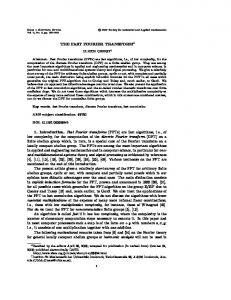
The harmonic distortion analysis prototype

Laptop

Lamp

Load Identification

LMBP

Figure 1. The meuserement system

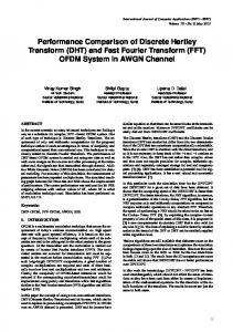
ARM microcontroller STM32F407VGT6 has large memory that sufficient to save the harmonic and power components calculation code. ARM microcontroller STM32F407VGT6 is equipped with 12 bit ADC to convert analog inputs into digital. In the ARM microcontroller STM32F407VGT6, 12 bit ADC has a fast conversion rate of 140 ns [17]. All these features are suitable for Harmonic and power components computation. The hall-effect sensor ACS712 is used for load current detection in the line. It has accuracy of 1.5% and frequency operation range of 80 kHz so allows to detect current harmonic distortion. Moreover, it provides an isolation of 2.1 kV so there is no need for additional protection [18]. AMC1100 is used for voltage detection in the line. It has accuracy of 0.5% and frequency operation range of 60 kHz so allows to detect voltage harmonic distortion. It provides an isolation 4.2 kV so there is no need for additional protection [19]. The hardware is shown in fig. 2.

calculation of the true rms values of voltage and current, the values of active power, reactive power and apparent power, the value of THD. The circuit of ZCD uses LM393 [20]. ZCD detects zero points for starting process of interrupt program and ending in the zero points so signal analysis can work on exactly one period. ZCD can find the values of phase between signals of voltage and current. In the fig. 3, voltage signal of 220 V is lowered corresponding specification of voltage sensor inputs by voltage divider with the values of 33K ohm and 220 ohm, respectively. Output signals of the voltage and current sensors starting in the zero points and toward to positive signals so output signals of LM393 toward to positive signals, conversely. Output signals of LM393 toward to IC not gate before toward as input signals of ARM microcontroller STM32F407VGT6. In the ARM microcontroller STM32F407VGT6, input signals of LM393 is programmed as interrupt whereas input signals of the voltage and current sensors is programmed as signal analysis calculation. 3.2. FFT Algorithm FFT is algorithm to decrease computational complexity of discrete fourier transform (DFT) [21], [22], [23], [24], [25]. Therefore, efficient computation can be obtained. The equation (1) shows DFT computation. N −1

X (k ) = ∑ x[n]e

−

j 2π kn N

, k, n=0,1,…,N-1

(1)

n=0

Where, X(k) = the output component in frequency domain x(n) = the input sample in time domain Fig. 2. Harmonic distortion analysis prototype

3.1. Zero Crossing Detector The implementation of zero crossing detector (ZCD) is to simplify the signal analysis as

The data sequence is divided in two sequence of length N/2. The samples are represented f1(n) and f2(n) for even samples and odd samples, respectively.

1082

Journal of Theoretical and Applied Information Technology 15th March 2017. Vol.95. No 5 © 2005 – ongoing JATIT & LLS

ISSN: 1992-8645

www.jatit.org 5V

E-ISSN: 1817-3195

3V

STM32F407VGT6

Source

ADC

AMC1100 33K ohm

5V

not gate

LM393 12K ohm

220 ohm

Interrupt 0 100 ohm 22 nF

5V

ADC

ACS712 5V

not gate

LM393 12K ohm

Interrupt 1 100 ohm

22 nF

5V

Load

Figure 3. Block diagram for hardware

j 2πnk N−1 X ( k ) = ∑ x(n)e N , n = 0, 1, ... N − 1 n=0

produces the highest harmonics. The voltage and current signals with random magnitudes and phase angles under different nonlinear loads can be expressed as [26], [27]:

N−1 N−1 nk + ∑ x ( n)⋅Wnk = ∑ x ( n)⋅WN N n even n odd =

( N/2)−1 ( N/2)−1 ∑ x (2m)⋅W2mk + ∑ h(2m+1)⋅W(2m+1) k N N m=0 m=0

=

( N/2)−1 k ( N/2)−1 ∑ x (2m)⋅Wmk + W ∑ x ( m)⋅W( m) k N/2 N/2 N m=0 m=0

k = F ( k ) + W F ( k ), N 2 1

H I ( t , γ ) = ∑ Ah (γ ) sin(2π fh t + θ h (γ )) (5) h=1

(2)

k = 0, ...., N − 1

With nk WN = e

j 2π nk N

(3)

F1(k) and F2(k) are periodic with period N/2. Therefore, FFT can be expressed as k S ( k ) = F1 ( k ) + WN F2 ( k ), N S (k +

N k = 0, 1, ..., 2 − 1

k ) = F ( k ) − W F ( k ), 1 N 2

Where, h is the harmonic order. Ah, fh, and θh are the amplitude, frequency and phase angle of the hth harmonic, respectively. Moreover, coefficient γ is a random variable that represents the timevarying behavior of distorted signal. The harmonic distortion value can be obtained from amplitude versus frequency that represents magnitude and phase of harmonic component individually. FFT provides amplitude frequency information to obtain the harmonic component. Indicator is used to show the value of harmonic distortion is total harmonic distortion (TDD) and voltage total harmonic distortion (THD). Equations (6) and (7) show indicator of current harmonic and voltage harmonic as: N

N (4) k = 0, 1, ..., 2 − 1

THDi =

2

2 ∑ In

n=2

N

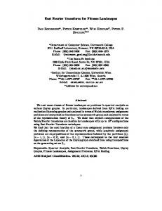
3.3. Harmonic Signature Characteristics Non-linear loads cause harmonic distortion. The harmonic distortion has characterization of the periodic signal. The harmonic characterization has significantly different signature, which can be considered as input to load identification. Fig. 4, shows the distinctive harmonic signatures of four types of non-linear loads. The air conditioner (AC)

THDV =

x100%

I1

(6)

2

∑ Vn

n= 2

V1

x100%

(7)

where, In and Ii are current magnitude in n-order and current magnitude in fundamental, respectively. Vn and Vi are voltage magnitude in n-order and voltage magnitude in fundamental, respectively.

1083

Journal of Theoretical and Applied Information Technology 15th March 2017. Vol.95. No 5 © 2005 – ongoing JATIT & LLS

ISSN: 1992-8645

www.jatit.org

E-ISSN: 1817-3195

the presence of loads based on their harmonic signature with high accuracy. LMBP is implemented using different numbers of neurons, and each case is trained for 100 iterations. LMBP is trained using harmonic data with combination of 14 different types of load. The detailed results of the load identification are listed in tables 2 and 3.

Fig. 4. Harmonic signature of various devices

4.

LEVENBERG MARQUARDT BACKPROPAGATION

LMBP is used to identify the existence of the device. Hidden layer uses different number of neurons, which used to evaluate performance LMBP. The number of neurons in the hidden layer are 10 neurons and 5 neurons. The number of input neuron into LMBP depends on the number of harmonics. In this research, harmonic order used to input neuron into LMBP is 1, 3, 5, 7, 9, 11, 15 and Total Harmonics Distortion (THD). In the LMBP method, the change weights

r

(∆) in the

(ω ) are obtained by solving [28], [29] 1 2

α ∆ = − ∇E

(8)

Information E is the mean-squared network error

E=

r 1 N r [ y ( xk ) − d k ]2 ∑ N k =1

(9)

Information N is the number of examples,

r y( xk )

example

is the network output appropriate to the

r

xk

and d k is the desired output for that

example. The elements of the by

α matrix

are given

 ∂y ( x ) ∂yr ( xk )  α ij = (1 + λδ ij )∑∑  r k  (10) ∂ω r  r =1 k =1  ∂ωi P

N

Information p is the number of outputs of the network. 5.

RESULT AND ANALYSIS

Application of the proposed algorithm is performed in two cases to evaluate the performance the proposed algorithm. Evaluation used to verify that load identification using LMBP can determine

Tables 2 and 3, show the average percentage error of the load identification using LMBP under different numbers of neurons. For combination 1, load identification with 10 neurons LMBP generate more accurate results compared to 5 neurons LMBP because the 10 neurons LMBP provide very minimal average percentage errors, which are 0.81% and 1.82%, respectively. For combination 2, load identification with 10 neurons LMBP generate more accurate results compared with 5 neurons LMBP because the 10 neurons LMBP provide very minimal average percentage errors, which are 0.57% and 1.27%, respectively. For combination 3, load identification with 10 neurons LMBP generate more accurate results compared with 5 neurons LMBP because the 10 neurons LMBP provide very minimal average percentage errors, which are 0.64% and 0.99%, respectively. For combination 4, load identification with 10 neurons LMBP generate more accurate results compared with 5 neurons LMBP because the 10 neurons LMBP provide very minimal average percentage errors, which are 0.17% and 1.09%, respectively. For combination 5, load identification with 10 neurons LMBP generate more accurate results compared with 5 neurons LMBP because the 10 neurons LMBP provide very minimal average percentage errors, which are 0.44% and 0.98%, respectively. For combination 6, load identification with 10 neurons LMBP generate more accurate results compared with 5 neurons LMBP because the 10 neurons LMBP provide very minimal average percentage errors, which are 0.11% and 0.35%, respectively. For combination 7, load identification with 10 neurons LMBP generate more accurate results compared with 5 neurons LMBP because the 10 neurons LMBP provide very minimal average percentage errors, which are 0.22% and 1.20%, respectively. For combination 8, load identification with 10 neurons LMBP generate more accurate results compared with 5 neurons LMBP because the 10 neurons LMBP provide very minimal average percentage errors, which are 1.70% and 3.12%, respectively.

1084

Journal of Theoretical and Applied Information Technology 15th March 2017. Vol.95. No 5 © 2005 – ongoing JATIT & LLS

ISSN: 1992-8645

www.jatit.org

E-ISSN: 1817-3195

Table 2. Identification result of the LMBP with 5 neurons Testing

Load 1 Load 2 Load 3 Load 4 Load 5 Load 6 Load 7 Load 8 Load 9 Load 10 Load 11 Load 12 Load 13 err(%) err(%) err(%) err(%) err(%) err(%) err(%) err(%) err(%) err(%) err(%) err(%) err(%)

Load 14 err(%)

1

1.08

1.49

2.52

1.63

0.34

0.27

0.62

2.52

4.33

0.75

0.01

2.12

0.56

2.10

2

0.71

0.92

1.03

0.96

0.99

0.11

1.66

3.14

4.29

0.85

0.26

2.11

0.86

0.05

3

0.13

0.93

0.43

0.54

1.10

0.07

1.81

3.18

0.45

1.51

0.85

0.96

0.60

1.95

4

3.10

1.54

0.00

0.75

1.27

0.57

1.23

3.87

1.58

1.25

1.33

3.13

0.00

1.09

5

4.10

1.46

0.97

1.55

1.20

0.71

0.65

2.87

0.01

0.49

0.82

1.50

1.40

1.19

Average

1.82

1.27

0.99

1.09

0.98

0.35

1.20

3.12

2.13

0.97

0.65

1.96

0.68

1.28

Table 3. Identification result of the LMBP with 10 neurons Testing

Load 1 Load 2 Load 3 Load 4 Load 5 Load 6 Load 7 Load 8 Load 9 Load 10 Load 11 Load 12 Load 13 err(%) err(%) err(%) err(%) err(%) err(%) err(%) err(%) err(%) err(%) err(%) err(%) err(%)

Load 14 err(%)

1

1.59

0.30

0.19

0.27

0.97

0.06

0.15

2.52

0.87

0.17

0.88

0.41

0.08

0.21

2

0.08

0.29

0.79

0.03

0.56

0.09

0.10

1.55

1.40

0.38

0.02

1.50

0.08

0.44

3

1.91

0.07

1.42

0.25

0.39

0.11

0.63

0.57

0.58

1.78

0.06

0.68

0.08

0.72

4

0.08

0.30

0.06

0.13

0.03

0.03

0.16

2.77

0.54

0.23

0.20

0.90

0.07

0.68

5

0.37

1.88

0.73

0.17

0.25

0.26

0.06

1.11

1.31

0.14

0.09

0.88

0.25

1.45

Average

0.81

0.57

0.64

0.17

0.44

0.11

0.22

1.70

0.94

0.54

0.25

0.88

0.11

0.70

For combination 9, load identification with 10 neurons LMBP generate more accurate results compared with 5 neurons LMBP because the 10 neurons LMBP provide very minimal average percentage errors, which are 0.94% and 2.13%, respectively. For combination 10, load identification with 10 neurons LMBP generate more accurate results compared with 5 neurons LMBP because the 10 neurons LMBP provide very minimal average percentage errors, which are 0.54% and 0.97%, respectively. For combination 11, load identification with 10 neurons LMBP generate more accurate results compared with 5 neurons LMBP because the 10 neurons LMBP provide very minimal average percentage errors, which are 0.25% and 0.65%, respectively. For combination 12, load identification with 10 neurons LMBP generate more accurate results compared with 5 neurons LMBP because the 10 neurons LMBP provide very minimal average percentage errors, which are 0.88% and 1.96%, respectively. For combination 13, load identification with 10 neurons LMBP generate more accurate results compared with 5 neurons LMBP because the 10 neurons LMBP provide very minimal average percentage errors, which are 0.11% and 0.68%, respectively. For combination 14, load identification with 10 neurons LMBP generate more accurate results compared with 5 neurons

LMBP because the 10 neurons LMBP provide very minimal average percentage errors, which are 0.70% and 1.28%, respectively. The results show that load LMBP to load identification is accurate and encouraging. Therefore, in the industrial, load identification using LMBP can be developed become smart meter to reduce energy consumption, observe power quality and energy audit. 6.

CONCLUSION

In this paper, LMBP is presented to identify the existence of the device in an electrical installation. LMBP is developed to identification of device based on the current harmonics. LMBP is implemented using different numbers of neurons, and each case is trained for 100 iterations. The results demonstrate that all load identification used 10 neurons LMBP generates more accurate results with a very minimal average percentage error of 0.11%. Therefore, the result of LMBP in the load identification is accurate and encouraging. Moreover, the result demonstrates that the average error percentage of the load identification using LMBP more accurate when the number of neurons increases. Future research will focus on experimental and extending the scope of the various loads.

1085

Journal of Theoretical and Applied Information Technology 15th March 2017. Vol.95. No 5 © 2005 – ongoing JATIT & LLS

ISSN: 1992-8645

www.jatit.org

REFRENCES: [1] D. Srinivasan, W. S. Ng, A.C. Liew, “NeuralNetwork-Based Signature Recognition for Harmonic Source Identification”, IEEE Trans. Power Del. Vol. 21, No. 1, Jan. 2006 [2] C. F. D. Nascimento, A. A. D. Oliveira, A. Goedtel, .P. J. A. Serni, “Harmonic Identification Using Parallel Neural Network in Single Phase System”, Applied Soft Computing, pp. 2178-2185, Nov. 2011 [3] IEEE std. 519-1992 “IEEE Recommended Practices and Requirement for Harmonic Control in Electrical Power Systems” [4] G. T. Heydt, “Identification of harmonic sources by a state estimation technique,” IEEE Trans. Power Del. vol. 4, no. 1, pp. 569-576, jan. 1989 [5] Z. P. Du, J. Arrilaga, N.R. Watson and S. Chen, “Identification of harmonic sources of power system using state estimation,” Proc. Inst. Elect. Eng., Gen., Transm. Distrib., vol. 146, pp. 7-12, 1999 [6] H. Ma and A. A. Girgis, “Identification and tracking of harmonic sources in a power system using a Kalman filter,” IEEE Trans. Power Del., vol.11, no. 3, pp. 1659–1665, Jul. 1996. [7] F. Sultanem, “Using appliance signatures for monitoring residential loads at meter panel level,” IEEE Trans. Power Del., vol. 6, no. 4, pp. 1380–1385, Oct. 1991. [8] G.W. Hart, “Nonintrusive appliance load monitoring,” Proc. IEEE, vol. 80, no. 12, pp. 1870–1891, Dec. 1992 [9] D. C. Robertson, O. I. Camps, J. S. Mayer, and W. B. Gish, Sr., “Wavelets and electromagnetic power system transients,” IEEE Trans. Power Del., vol. 11, no. 2, pp. 1050–1056, Apr. 1996. [10] A. I. Cole and A. Albicki, “Data extraction for effective non-intrusive identification of residential power loads,” in Proc. IEEE Instrument. Meas. Technol. Conf., 1998, pp. 812–815 [11] A. I. Cole and A. Albicki, “Algorithm for nonintrusive identification of residential appliances,” in Proc. IEEE Int. Symposium Circuits Syst., 1998, pp. 338–341 [12] R. K. Hartana and G. G. Richards, “Constrained neural network-based identification of harmonic sources,” IEEE Trans. Ind. Appl., vol. 29, no. 1, Pt. 1, pp. 202–208, Jan./Feb. 1993. [13] Lera, G., Pinzolas, M., “Neighborhood Based Levenberg Marqaurdt Algorithm for Neural

E-ISSN: 1817-3195

Network Training”, IEEE Trans. on Neural Network, Vol. 13, No. 5, Sep. 2002 [14] Saini, L.M., Soni, M.K., “Artificial Neural Network Based Peak Load Forecasting Using Levenberg-Marquardt and Quasi-Newton Methods”, IET Gen. Trans. and Dist., Vol. 149, pp. 578 – 584, 2012 [15] Wilamowski, B.M., Yu, H., “Improved Computation for Levenberg-Marquardt Training”, IEEE Trans. On Neural Network, Vol.21, No.6, Jun. 2010 [16] Toledo, A., Pinzolas, M., Ibarrola, J.J., Lera, G., “Improvement of the Neighborhood Based Levenberg-Marquardt Algorithm by Local Adaptation of the Learning Coefficient”, IEEE Trans. On Neural Network, Vol. 16, No. 4, Jul. 2005 [17] STM32F407VGT6. [online]. Available. https: http://www.st.com/stwebui/static/active/en/resource/technical/docum ent/datasheet/DM00037051.pdf [18] Voltage transducer AMC1100. [online]. Available: www.ti.com/lit/ds/ symlink/amc1100.pdf [19] Current Transducer ACS712. [online]. Available. https://www.mpja.com /download/acs712.pdf [20] LM393. [online]. http://www.ti.com/lit/ds/symlink/lm393.pdf [21] Y. A. Familiant, H. Jing, K. A. Corzine, and M. Belkhayat, “New techniques for measuring impedance characteristics of three-phase AC power systems,” IEEE Trans. Power Electron., vol. 24, no. 7, pp. 1802–1810, Jul. 2009 [22] D. Agrez, “Weighted multipoint interpolated DFT to improve amplitude estimation of multi frequency signal,” IEEE Trans. Instrument Meas., vol. 51, no. 2, pp. 287–292, Apr. 2002\ [23] D. Belega and D. Dallet, “Amplitude estimation by a multipoint interpolated DFT approach,” IEEE Trans. Instrument Meas., vol. 58, no. 5, pp. 1316–1323, May 2009 [24] F. Zhang, Z. Geng, W. Yuan, “The Algorithm of interpolating Windowed FFT for harmonic Analysis of electric Power System”, IEEE Trans. Power Del., Vol. 16, No. 2, Apr. 2001 [25] H.Qian, R. Zhao, T. Chen, “Interhamonics Analysis Based on Interpolating Windowed FFT Algorithm” IEEE Trans. Power Del, Vol. 22, no. 2, Apr. 2007 [26] C. F. Nascimento, A. A. Oliveira Jr. A. Goedtel. A. B. Dietrich, “Harmonic Distortion

1086

Journal of Theoretical and Applied Information Technology 15th March 2017. Vol.95. No 5 © 2005 – ongoing JATIT & LLS

ISSN: 1992-8645

www.jatit.org

Monitoring for Nonlinear Loads Using NeuralNetwork-Method”, Applied Soft Computing, 2013 [27] S. Nath, P. Sinha, S. K. Goswami, “A Wavelet Based Novel Method for the Detection of Harmonic Sources in Power Systems”, Electrical Power and Energy Systems, 2012 [28] A. Tjahjono, D.O. Anggriawan, A. Priyadi, M. Pujiantara, M.H. Purnomo, “Digital Overcurrent Relay with Conventional Curve Modeling Using Levenberg Marquardt Backpropagation”, IEEE International Seminar on Intelligent and Its Applications, 2015 [29] I.S. Faradisa, D.O. Anggriawan, T.A. Sardjono, M.H. Purnomo, “Identification of Phonocardiogram Signal Based on STFT and Marquardt Lavenberg Backpropagation” IEEE International Seminar on Intelligent and Its Applications, 2016

1087

E-ISSN: 1817-3195