Harvey's Average Polynomial Time Algorithms - UnTruth.org

. .

Harvey’s Average Polynomial Time Algorithms Joshua E. Hill Department of Mathematics, University of California, Irvine

Math 239B Arithmetic Geometry January 6 and 8, 2014 http://bit.ly/198j5HY v1.01, compiled March 18, 2014

1 / 46

Talk Outline

1

Introduction

2

The Sieve of Eratosthenes

3

Searching for Wilson Primes

4

5

Computing Zeta Functions of Arithmetic Schemes Modulo Many Primes Conclusion

2 / 46

Introduction Outline

1

Introduction GOOOOOOOOOOOOOOOOOOOOOOOOOOOOALS! Time Complexity Notes

2

The Sieve of Eratosthenes

3

Searching for Wilson Primes

4

5

Computing Zeta Functions of Arithmetic Schemes Modulo Many Primes Conclusion

3 / 46

Subsection 1 GOOOOOOOOOOOOOOOOOOOOOOOOOOOOALS!

4 / 46

A Tale of Two Complexities

I

Calculating the number of elements can be hard.

I

We often don’t have general algorithms that run in polynomial time (with respect to p). We have two basic classes of responses:

I

Make the problem much smaller (extra hypotheses that impose some nice structure.) Make the problem much larger.

5 / 46

Say What!?!

Make the problem much...

6 / 46

Say What!?!

Make the problem much...

Larger

7 / 46

Say What!?!

Make the problem much...

Larger (and then hope for a reasonable amortized runtime.)

8 / 46

So it begins...

We’ll look at a few examples: I

The Sieve of Eratosthenes

I

Searching for Wilson Primes

I

Calculate the zeta function for reductions of an arithmetic scheme mod all primes less than some bound.

9 / 46

Papiere, Bitte

We’ll be exploring the following papers (the third provides the basic algorithm used in the second): I

Edgar Costa, Robert Gerbicz, and David Harvey, A Search for Wilson Primes.

I

David Harvey, Computing Zeta Functions of Arithmetic Schemes

10 / 46

Subsection 2 Time Complexity Notes

11 / 46

Big-O Notation (and Family) I

I

We have two eventually positive real valued functions A; B W N k ! R. Take x as an n-tuple, with x D .x1 ; : : : ; xn / We’ll write jxjmin D mini xi .

. Definition . A.x/ D O.B.x// if there exists a positive real constant C and an integer N so that if jxjmin > N then A.x/  CB.x/. (i.e. A is bounded above by B .asymptotically.) . Definition . A.x/ D o.B.x// if for all positive real constants C there is an integer N so that if jxjmin > N then A.x/  CB.x/. (i.e. A is dominated by B asymptotically.) . 12 / 46

“When I Use a Word...”

. Definition . An algorithm is considered polynomial time if it is time complexity k .O.x / where k is a fixed positive integer and x is the input length. . Definition . An algorithm is considered exponential time if it is time complexity xk .O.2 / where k is a fixed positive integer, and x is the input length.

13 / 46

The Sieve of Eratosthenes

1

Introduction

2

The Sieve of Eratosthenes

3

Searching for Wilson Primes

4

5

Computing Zeta Functions of Arithmetic Schemes Modulo Many Primes Conclusion

14 / 46

The Algorithm

I

Determine the largest number you want to test, N.

I

Make a bit-array (initialized to all 0s) of length N.

I

Mark 1 as not prime (set the first entry to 1).

I

Let k D 2

I

Until k is larger than

jp k N , do the following:

Mark every positive integer multiple of k greater than k and less than or equal to N as not prime (set their corresponding bit array entries to 1). Let k be the next entry marked as prime. I

The values marked as prime are the primes less than or equal to N.

15 / 46

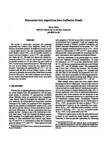
An Example of the Sieve

Figure : Sieve of Eratosthenes, N D 100 16 / 46

Computational Complexity I

k can only be a prime number.

I

There are fewer than bN=kc values excluded for each value of k.

I I

Each step is just an addition of a value of size O.log N/.

The total number of excluded values, d, is thus (by Mertens’ theorem) X d bN=kc D O.N log log N/ p k N k prime

I

We can then read out the primes by looking for 0 bits in the bitstring in O.N/.

I

The runtime is thus O.d log N/ D O.N log N log log N/.

I

This algorithm requires O.d log N/ storage.

I

Even if we don’t assume a RAM model (and instead use a Turing model) we can get a similar result using sorting. 17 / 46

A Note on O .N/

I


O .N/ D O elog N is clearly exponential in log N (the size of N).

I

O.N log N log log N/ is exponential in the size of N.

I

We got .N/  N= log N primes from the algorithm.

I

The amortized runtime per-prime is thus O.log2 N log log N/, which is polynomial in the input size.

18 / 46

A Note on O .N/

I


O .N/ D O elog N is clearly exponential in log N (the size of N).

I

O.N log N log log N/ is exponential in the size of N.

I

We got .N/  N= log N primes from the algorithm.

I

I

The amortized runtime per-prime is thus O.log2 N log log N/, which is polynomial in the input size. Jazz Hands!

19 / 46

Search for Wilson Primes Outline

1

Introduction

2

The Sieve of Eratosthenes

3

Searching for Wilson Primes

4

5

Computing Zeta Functions of Arithmetic Schemes Modulo Many Primes Conclusion

20 / 46

Wilson Primes

I

I

By Wilson’s Theorem, we know that p is prime if and only if .p 1/Š  1 .mod p/. For a prime p, define wp D ..p

1/Š C 1/=p .mod p/.

. Definition . A Wilson Prime is a prime where wp  0 .mod p/, or equivalently when .p 1/Š  1 .mod p2 /. . I

There are three known Wilson Primes: 5, 13, and 563.

I

It is conjectured that there are an infinite number of Wilson Primes.

21 / 46

WILSON!!!

I

In general, the tests to see if a prime p is a Wilson prime are exponential in the size of p.

I

By using a dynamic programming technique called memoization, one can (in aggregate) make this calculation more efficient.

I

Idea: As p varies, we repeat quite a lot of arithmetic in calculating .p 1/Š.

22 / 46

I Wanted to be... A LUMBERJACK!

I

We seek Wilson primes less than or equal to some fixed N.

I

We first need to find all the primes up to N.

I

We use the Sieve of Eratosthenes, which we have seen runs in O.N log N log log N/.

23 / 46

Trees for the Forest: The Larch

I

I

I

We’ll break the interval Œ1; N into 2i roughly equal intervals:   N N Ui;j D k 2 Z j j i < k  .j C 1/ i 2 2 ` The recurrence relation Ui;j D UiC1;2j UiC1;2jC1 provides a tree structure. ˇ ˇ Let d D dlog Ne. Note ˇUd;j ˇ is either 0 or 1 for all j. 2

24 / 46

Trees for the Forest: The Pine I

Multiply together the elements in each set: Y Ai;j D k k2Ui;j

I I I

I

By the recurrence relation for Ui;j we get Ai;j D AiC1;2j
AiC1;2jC1 . Ad;j is either 1 (when Ud;j D ;) or k (when Ud;j D fkg).

The Ai;j product tree can be computed from bottom (i D d) to top (i D 0) using the above recurrence relation. Elements in the ith level are O.2 i N log N/ bits long.

I

For fixed i, all the Ai;j can be computed in work factor 2i .2 i N log N/ log1C N.

I

There are log2 N levels, so the cost for computing the Ai;j tree is N log3C N. 25 / 46

Trees for the Forest: The Redwood

I

Multiply together the squares of the prime elements in each set: Y Si;j D p2 p2Ui;j p prime

I

The characteristics of Si;j are similar to those of Ai;j .

I

By the recurrence relation for Ui;j we get Si;j D SiC1;2j
SiC1;2jC1 .

I

The Si;j product tree can be computed from bottom (i D d) to top (i D 0) using the above recurrence relation.

I

Elements in the ith level are at most O.2 i N log N/ bits long.

I

The cost for computing the Si;j tree is less than N log3C N.

26 / 46

Trees for the Forest: The Sequoia I

Calculate factorial parts and reduce. Wi;j D

I I I I

I

I

Y

Ai;j

0r 1. Given E1 ;


; EN 1 (with entries bounded suitably by ), Qpa 1set of m  m matrices with entries in ZŒk=kˇ . We can then compute iD1 Ei .mod p / for all primes p < N 1C 3 in . time m ˇ. C /N log N log .ˇN/.

40 / 46

Same Old Story, Not Much to Say I

Happily, this is very similar to the instance where we searched for Wilson Primes.

I

` D dlog2 Ne

I

These all form binary trees in exactly the same way as before.

I

Si;t (loosely) partitions the integers 0; : : : ; N roughly equal size.

I

Pi;t contains the primes of Si;t .

I

The modulus tree is defined Mi;t D Q The value tree Vi;t D j2Si;t Ej .

I

Q

p2Pi;t

1 into 2i sets of

p .

I

The accumulating remainder tree is Ai;t D Vi;t 1 Vi;t .mod Mi;t /.

2


Vi;0

I

This last tree is constructed using the recurrence relations AiC1;2t D Ai;t .mod MiC1;2t / and AiC1;2tC1 D ViC1;2t Ai;t .mod MiC1;2tC1 /. 41 / 46

Hearts are Broken, Everyday

I

If we average this cost over all the primes less than N, we get a polynomial algorithm.

I

This algorithm (not just the many-p case) is the fastest known algorithm of this type.

42 / 46

Section 5 Conclusion

43 / 46

Jazz Hands!

I

This “amortized cost” style algorithm allows for use of a broader class of tools.

I

For some styles of problem, we really do mainly care about the cost-per-result, rather than the cost of the entire operation.

I

These algorithms are still “slow” with respect to input size.

44 / 46

Thank You! 45 / 46

Bibliography

I

Edgar Costa, Robert Gerbicz, and David Harvey, A Search for Wilson Primes.

I

David Harvey, Computing Zeta Functions of Arithmetic Schemes

46 / 46