Proceedings of ACIVS 2002 (Advanced Concepts for Intelligent Vision Systems), Ghent, Belgium, September 9-11, 2002
POLYNOMIAL TIME CLUSTERING ALGORITHMS DERIVED FROM BRANCH-AND-BOUND TECHNIQUE Pasi Fränti and Olli Virmajoki
[email protected],
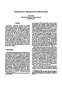
[email protected] University of Joensuu, Department of Computer Science, P.O. Box 111, FIN-80101 Joensuu, FINLAND A branch-and-bound technique has been proposed in [8] based on the merging approach described above. It is easy to see that any clustering can be produced by a series of merge operations. Every merge reduces the number of clusters by one. It therefore takes exactly N-M steps to generate a clustering with M groups from the set of N data vectors. Optimal clustering can be found by considering all possible merge sequences and finding the one that minimizes the optimization function. This can be implemented as a branch-and-bound technique, which uses search tree for finding the optimal clustering. The relation of the branch-and-bound technique and the PNN method is demonstrated in Fig. 1. The complexity of the branch-and-bound technique, however, is exponential and the practical usability is therefore strongly limited to small size problem instances only. In this paper, we propose two sub-optimal variants that do not guarantee the optimality of the result but they work in polynomial time. The first algorithm, Piecewise optimization, divides the problem into a series of smaller sub problems that are solved optimally. The input at each stage of the algorithm is N clusters (whole data set in the beginning), and the output is the optimal clustering to N-Z clusters, where Z is a parameter of the algorithm. The result is then input to the same procedure, and the process is repeated until the desired number of M clusters is reached. The second algorithm, Look-ahead optimization, generates complete search tree to the level Z and searches for the optimal clustering of N-Z clusters. Instead of moving to the local optimum at the level Z, it proceeds only one level in the tree along the path towards to the direction of the local optimum. After this, a completely new search tree is generated starting from the level N-1. The process is repeated N-M times.
Abstract Optimal clustering can be solved using branch-and-bound technique. The algorithm has exponential time complexity and, therefore, only very small size problem instances can be solved in practice. On the other hand, the branch-and-bound technique provides useful insight to the problem itself, which can be utilized in designing of practical clustering algorithms. In this paper, we propose two sub-optimal but polynomial time algorithms derived from the branch-and-bound technique. The proposed algorithms generate only partial search tree, which are solved optimally. The final solution is achieved by a series of locally optimal steps.
1.
INTRODUCTION
Clustering is an important problem that must often be solved as a part of more complicated tasks in pattern recognition, image analysis and other fields of science and engineering [1, 2, 3, 4]. Clustering aims at partition a given set of N data vectors into M groups so that similar vectors are grouped together and dissimilar vectors to different groups. The clustering task is usually formalized as a combinatorial optimization problem, in which the goal is to find the partition that minimizes a given cost function. The clustering problem in its combinatorial form has been shown to be NP-complete [5]. No polynomial time algorithm is known to find the optimal solution. Therefore, we have to content ourselves with sub-optimal solutions obtained by heuristic algorithms. Despite known limitations implicated by the NP-completeness, solving the optimal clustering problem has some theoretical interest that provides also new insight to the problem itself. Agglomerative clustering is heuristic approach for generating the clustering hierarchically. The process starts by initializing each data vector as its own cluster. Two clusters are merged at each step and the process is repeated until the desired number of clusters is obtained. Ward’s method [6] selects the cluster pair to be merged so that it increases the given objective function value least. In the vector quantization context, this is known as the pairwise nearest neighbor (PNN) method due to [7]. In the rest of this paper, we denote it as the PNN method.
2.
CLUSTERING BY BRANCH-AND-BOUND
Next we give formal description of the clustering problem, and recall the PNN method. The branch-and-bound technique is then given as a method to generate minimum
S00-1
Proceedings of ACIVS 2002 (Advanced Concepts for Intelligent Vision Systems), Ghent, Belgium, September 9-11, 2002
redundancy search tree. A bounding criterion is also discussed.
1'st merge
AB
AC
AD
2'nd merge
AE
AEB
BC
AEC AED
BD
BE
BC
BD
AEBC
AED
CD
CE
2.2. Pairwise nearest neighbor method The pairwise nearest neighbor (PNN) method [6, 7] generates the clustering hierarchically using a sequence of merge operations. In each step of the algorithm, the number of the clusters is reduced by merging two nearby clusters:
DE
The cost of merging two clusters sa and sb is the increase in the MSE-value caused by the merge. It can be calculated using the following formula [7]:
CD
N= 5 M=2 1'st merge
BCD
3'rd merge
2'nd and 3'rd merge
d a ,b =
B A E
D
2.1. Definition of clustering problem The clustering problem is defined here as follows. Given a set of N data vectors X={x1, x2, …, xN}, partition the data set into M clusters such that similar vectors are grouped together and dissimilar vectors to different groups. Partition P={p1, p2, …, pN } defines the clustering by giving for each data vector the cluster index of the group where it is assigned to. A cluster sa is defined as the set of data vectors that belong to the same partition a:
{
}
1 N × å xi - c pi N i =1
(4)
The idea of the PNN can be generalized to a branch-andbound technique by generating the clustering by a sequence of merge operations as proposed in [8]. It is easy to see that any clustering can be produced by a sequence of merge operations. Every merge operation reduces the number of clusters by one. It therefore takes exactly N-M steps to generate a clustering with M clusters, independent of the clustering and of the order of the merge operations. For example, consider the example shown in Fig. 1, in which we have five data points {A, B, C, D, E}. The resulting clustering can be generated by the following three merge operations: Initial: {A} {B} {C} {D} {E} Step 1: {AE} {B} {C} {D} Step 2: {AE} {BC} {D} Step 3: {AE} {BCD} All possible merge sequences can be represented as a search tree. The root of the tree represents the starting point, in which every data vector is assigned to its own cluster (N clusters), and its descendants represent all possible clusterings to N-1 clusters. In general, every node represents a single clustering with m clusters and its children represent the clusterings that have been produced by merging any two of the m existing clusters. The optimal clustering can be found by systematic search from the tree.
(1)
2
2
2.3. Branch-and-bound technique
The clustering is then represented as the set S={s1, s2, ..., sM}. The clusters are sometimes also represented as their centroids: C={c1, c2, …, cM}. The most important choice is the cost function f for evaluating the goodness of the clustering. When the data vectors are in Euclidean space, a commonly used function is the mean square error between the data vectors and their nearest cluster centroids. Given a partition P and the cluster representatives C, it is calculated as: MSE (C , P ) =
na nb × ca - cb na + nb
where na and nb are the corresponding cluster sizes. The PNN applies local optimization strategy: all possible cluster pairs are considered and the one increasing the distortion least is chosen. A single merge step of the PNN is optimal but there is no guarantee of optimality of the final clustering resulting from a series of locally optimal merge steps. The time complexity of the PNN varies from O(N2) to O(N3) depending on the implementation and data set [9].
C
Fig. 1. Illustration of the PNN as a search tree.
sa = xi pi = a
(3)
sa ¬ sa È sb
(2)
The choice of the function depends on the application and there is no general solution to be used. However, once the objective function is decided the clustering problem can be formulated as a combinatorial optimization problem.
S00-2
Proceedings of ACIVS 2002 (Advanced Concepts for Intelligent Vision Systems), Ghent, Belgium, September 9-11, 2002
AB
ABC ABD ABE CD
ABCD
DE
ABCE
CDE
CE ABDE
AC
CE
DE
ACD ACE BD
ACDE
BE
AD
BE
DE
BDE
ADE
BC
BC
BCE
AE
BE
BC
BD
BC
CD
BCD
BCD BCE
BD
BDE
BCDE
BD
CD
Fig. 2. Example of non-redundant search tree. Branches that do not have any valid clustering have been cut out. the permutation criterion (5). The non-redundant search tree is illustrated in Fig. 2. The criterion (5) removes redundant clusterings but there still exist partial branches that cannot be completed. For example, after the merge sequence (AB) ® (CE) there are no more valid merges left because the permutation criterion does not allow to add anymore vectors in the cluster (AB), and because the merge (CE)+(D) would break the intracluster order. Fortunately, such branches can be eliminated using rather simple bounds for the permutation loop as derived in [8]. The pseudo code is formulated in Fig. 3.
2.4. Permuting non-redundant search tree We consider next a single cluster represented as a list of the data vectors, and merge operation as the catenation of the two lists. For example, the clustering in Fig. 1 is represented as the pair (AE) (BCD), and their merge as (AE) + (BCD) = (AEBCD). The search tree includes a lot of redundancy as the same clustering can be constructed by many different order of the merge operations. For example, the clustering (AE) (BCD) can be reached by six different merge sequences, of which two are shown in Table 1. We must therefore limit the permutation of the search paths in the tree. Table 1: Example of generating clustering (AE) (BCD) via two different merge sequences. Sequence 1:
Sequence 2:
(A) (B) (C) (D) (E) (AE) (B) (C) (D) (AE) (BC) (D) (AE) (BCD)
(A) (B) (C) (D) (E) (A) (BC) (D) (E) (A) (BCD) (E) (AE) (BCD)
Branch-and-bound(X, M) ® S; FOR i¬1 to N DO si ¬ {xi}; S ¬ BB(S, 1, 2, M); BB(S0, a0, b0, M) ® Sbest, MSEbest; MSEbest ¬ ¥; IF |S0| = M THEN RETURN S0, MSE(S0); FOR a ¬ a0 to M bmin ¬ b0 IF a=a0 THEN ELSE bmin ¬ a+1 FOR b ¬ bmin to |S0|
The redundancy of the search paths can be removed as follows. The algorithm permutes the cluster pair sa and sb in a predefined order so that the index of the first cluster (A) is always monotonically non-decreasing during the process, and that the index of the second cluster is greater that of the first clusters: b > a. In other words, if we have merged clusters sa0 and sb0 at the previous level, we should consider only cluster pairs sa and sb such that a ³ a0. This can be formalized as follows:
(s a , sb ) : a ³ a0 Ùb > a
S ¬ S0 ; S ¬ Merge(S, sa, sb); S, mse ¬ BB(S, a, b, M); IF mse < MSEbest THEN MSEbest ¬ mse; Sbest ¬ S; END-IF END-FOR END-FOR
(5)
RETURN Sbest, MSEbest;
where a0 is the index of the first cluster in the previous merge. Any clustering {s1, s2, ..., sm} can then be generated by constructing the clusters one by one in the order from s1 to sm. Furthermore, there is no other merge sequence that could construct the same clustering without contradicting
Fig. 3. Algorithm for generating non-redundant search tree.
S00-3
Proceedings of ACIVS 2002 (Advanced Concepts for Intelligent Vision Systems), Ghent, Belgium, September 9-11, 2002
2.5. Bounding criterion
3.2. Look-ahead optimization
It is also possible to bound the search if we know that the current branch cannot lead to a better solution than the best solution found so far. The bounding is based on the fact that every merge operation increases the MSE-value of the solution. Thus, when we have generated the first solution in the search tree, we can use its MSE-value as the upper limit for the optimal solution. Other branches of the tree can then be terminated if the following condition is true:
The Piecewise optimization traverses the search tree through local optima. At each stage of the algorithm, the last merge is the most critical because the algorithm can see only one level forward in the tree. Slightly better but Z times slower variant, denoted as Look-ahead optimization, is therefore proposed as follows. As in the Piecewise optimization, the Look-ahead optimization generates a complete search tree down to the level Z, and then searches for the optimal clustering with N-Z clusters. Instead of moving to this local optimum at the level Z, the algorithm proceed only one level in the tree along the path towards the direction of the local optimum. After the single step, a completely new search tree is re-generated starting from the level N-1. The process is repeated N-M times as illustrated in Fig. 6. This variant is less critical for the local minima. As a drawback, the time complexity of the algorithm is Z times that of the previous variant. With Z-values larger than 2, we would also do unnecessary work as a part of the search tree would be re-generated several times. In practice, the algorithm can be realized only with very small values of Z.
MSEt ³ MSEmin
3.
(6)
POLYNOMIAL TIME VARIANTS
We introduce next two sub-optimal variants of the branchand-bound technique. The algorithms do not guarantee the optimality of the result but they work in polynomial time. 3.1. Piecewise optimization The original optimization problem is divided into a series of smaller sub problems that are solved optimally. The input at each stage of the algorithm is N clusters (whole data set in the beginning), and the output is the optimal clustering to N-Z clusters, where Z is a parameter. The result is then input to the same procedure, and the process is repeated until the desired number of M clusters is reached. The method is denoted as Piecewise optimization, and it is illustrated in Fig. 4.
N clusters Z merge steps N - Z clusters
N - 2Z clusters
If the size of a single sub-problem is Z, we need é(N-M)/Zù stages in the algorithm. The quality of the result depends on the parameter Z; greater values give better clustering result at the cost of longer run time. The extreme case is when we set Z=N-M, which would result to the same algorithm as the branch-and-bound technique in Section 2. By setting Z=1, on the other hand, the method would be the same as the original PNN method. The pseudo code of the Piecewise optimization is shown in Fig. 5. At the starting point of the algorithm when we have N clusters as the input, we have O(N2) possible merge operations to be considered. Two subsequent merge operations results in O(N4) different solutions. In general, the time complexity of z subsequent merge operations is O(N2Z), and the overall Piecewise algorithm is O(N×N2Z). The algorithm works in polynomial time when Z is small enough to be considered as a constant. On the other hand, the time complexity increases exponentially as a function of Z. The algorithm is therefore useful only with very small values of Z, for example Z=2, or Z=3.
N - 3Z clusters
M clusters Final result
Fig. 4. Illustration of the Piecewise optimization. The starting points at each step are shown as white dots. PiecewiseOptimization(X, M, Z) ® S; FOR i¬1 to N DO si ¬ {xi}; REPEAT size ¬ max(M, |S|-Z); S ¬ BB(S, 1, size, ¥); UNTIL |S| = M;
Fig. 5. Piecewise optimization algorithm.
S00-4
Seconds
Proceedings of ACIVS 2002 (Advanced Concepts for Intelligent Vision Systems), Ghent, Belgium, September 9-11, 2002
Local minima
3000 2500 2000 1500 1000 500 0
B&B with bounding criterion
3
5
7
9
11
B&B
13
15
17
Size of the data set
Fig. 7. The dependency of time from the size of data with M=2 clusters.
Final result
Fig. 6. Illustration of the Look-Ahead optimization. The starting points at each step are shown as white dots. EXPERIMENTAL RESULTS
Seconds
4.
We consider first simulated data sets in order to find out how large clustering problems the optimal branch-andbound technique can solve. The results are summarized in Fig. 7-8 with different number of clusters using Pentium 450 MHz computer for simulated data set. The algorithm is fastest when the number of clusters is set small (M=2), or large (M=9). These correspond to the situations, in which the number of possible solutions is smallest. The use of early termination improves the algorithm but the improvement is only marginal. We conclude that the practical usability of the optimal branch-and-bound algorithm is limited to very small size problem instances only. Similar results are given also to the polynomial time variants in Fig. 9. The algorithms are performed for a simulated data set with 15 clusters. The size of the data set is varied by randomly subsampling source data set of 1000 vectors. The polynomial time variants are faster and can process larger data sets than the optimal branch-andbound technique. Only small sub tree sizes (Z=2,3) were applied. The qualities of the sub-optimal variants are compared in Table 2 with other heuristic clustering methods. The random clustering is obtained by randomly selecting M data vectors and use them as cluster representatives, and then partition the rest of the data set by minimizing Euclidean distance from the data vectors to the cluster representatives. K-means is an iterative clustering algorithm, which is also known as the GLA in vector quantization context due to [11]. The PNN is implemented as in [9], and the RLS refers to the Randomized Local Search method [12], which is one of the best heuristic clustering algorithms in terms of quality.
12000 10000 8000 6000 4000 2000 0
B&B with bounding criterion
B&B
10 11 12 13 14 15 16 17 18 Size of the data set
Fig. 8. The dependency of time from the size of data with M=9 clusters. 2000
Look-ahead (Z =3)
Look-ahead (Z =2)
Seconds
1500 1000
Piecewise (Z =3) Piecewise (Z =2)
500 0 30
40
50
60
70
80
90 100 110 120
Size of the data set
Fig. 9. The effect of the problem size to the run time in the case of the polynomial time variants (M=15).
In comparison to the PNN, the polynomial time variants (Piecewise and Look-ahead) manage to produce better clustering in two cases (N=70, 80) but the difference is marginal. For the rest of the data there are no differences between the PNN and branch-and-bound variants. The RLS, on the other hand, gives somewhat better results than the PNN and BB. It is noted that the optimality of the results is not known but it is expected that the RLS results are close to optimum.
S00-5
Proceedings of ACIVS 2002 (Advanced Concepts for Intelligent Vision Systems), Ghent, Belgium, September 9-11, 2002
Table 2: Performance comparison for the simulated data set (N=30..100). The values are mean square errors (´109). Method:
N=30
N=40
N=50
N=60
N=70
N=80
N=90
N=100
Random clustering
2.996
2.914
7.093
4.181
5.399
4.940
4.545
4.062
K-means [12]
0.948
1.081
1.108
1.541
1.647
1.614
1.628
1.837
PNN [8]
0.396
0.573
0.992
1.181
1.246
1.225
1.274
1.373
BB: Piecewise (Z=2)
0.396
0.573
0.992
1.181
1.240
1.206
1.274
1.373
BB: Look-ahead (Z=2)
0.396
0.573
0.992
1.181
1.240
1.206
1.274
1.373
RLS [13]
0.396
0.573
0.992
1.141
1.203
1.169
1.238
1.335
is noted more tests should be performed to obtain more conclusive results.
Finally, we compare the performance of different clustering methods for a standard clustering test problem SS2 of [10], pp. 103-104. The data set contains 89 postal zones in Bavaria (Germany) and their attributes are the number of self-employed people, civil servants, clerks and manual workers in these areas. The attributes are normalized to the scale [0, 1] according to their minimum and maximum values. The results in Table 3 indicate that the Piecewise and Look-ahead algorithms can improve over the PNN and the K-means but at the cost of significant increase in run time. The results, however, are still worse than that of the RLS. Moreover, the slowness of the algorithms may restrict their use in the case of larger data sets.
6.
[1] Everitt BS, Cluster Analysis, 3rd Edition. Edward Arnold / Halsted Press, London, 1992. [2] Kaufman L, Rousseeuw PJ, Finding Groups in Data: An Introduction to Cluster Analysis. John Wiley Sons, New York, 1990. [3] Dubes R, Jain A, Algorithms that Cluster Data. Prentice-Hall, Englewood Cliffs, NJ, 1987. [4] A. Gersho and R.M. Gray, Vector Quantization and Signal Compression. Kluwer Academic Publishers, Dordrecht 1992.
Table 3: Performance comparison for the data set SS2 (N=89) [10]. The values are mean square errors (´109). Method:
Error:
Time:
Random clustering
1.760
»0s
K-means [11]
1.140
»0s
PNN [9]
0.336
»0s
BB: Piecewise (Z=2)
0.323
342 s
BB: Piecewise (Z=3)
0.336
1061 s
BB: Piecewise (Z=4)
0.323
4851 s
BB: Look-ahead (Z=2)
0.323
652 s
BB: Look-ahead (Z=3)
0.316
3129 s
RLS [12]
0.313
»0s
5.
REFERENCES
[5] M.R. Garey, D.S. Johnson, H.S. Witsenhausen, "The complexity of the generalized Lloyd-Max problem". IEEE Transactions on Information Theory, 28 (2), 255-256, March 1982. [6] J.H. Ward, "Hierarchical grouping to optimize an objective function", J. Amer. Statist.Assoc., 58, 236-244, 1963. [7] W.H. Equitz, "A new vector quantization clustering algorithm", IEEE Transactions on Acoustics, Speech, and Signal Processing 37 (10), 1568-1575, October 1989. [8] P. Fränti, O. Virmajoki and T. Kaukoranta, "Branch-andbound technique for solving optimal clustering", Int. Conf. on Pattern Recognition (ICPR’02), Québec, Canada, August 2002. (to appear) [9] P. Fränti, T. Kaukoranta, D.-F. Shen and K.-S. Chang, "Fast and memory efficient implementation of the exact PNN", IEEE Transactions on Image Processing, 9 (5), 773-777, May 2000.
CONCLUSIONS
[10] H. Späth, Cluster Analysis Algorithms for Data Reduction and Classification of Objects, Ellis Horwood Limited, West Sussex, UK, 1980.
We have introduced two polynomial time algorithms that were analytically derived from the optimal branch-andbound technique. The algorithms offer good compromise between the optimal algorithm and the PNN. They can operate with larger data sets than the optimal branch-andbound technique and, on the other hand, give better results than the PNN in terms of quality. However, the methods were still outperformed by the best competitor (the RLS). It
[11] Y. Linde, A. Buzo and R.M. Gray, "An Algorithm for Vector Quantizer Design", IEEE Transactions on Communications, 28 (1), 84-95, January 1980. [12] P. Fränti and J. Kivijärvi, "Randomized local search algorithm for the clustering problem", Pattern Analysis and Applications 3(4): 358-369, 2000.
S00-6