HBBA: Hybrid Algorithm for Buffer Allocation in Tandem Production ...

HBBA: Hybrid Algorithm for Buffer Allocation in Tandem Production Lines

Alexandre DOLGUI 1,†, Anton V. EREMEEV 2, and Viatcheslav S. SIGAEV 3 1

Division for Industrial Engineering and Computer Sciences, Ecole des Mines de Saint Etienne, FRANCE, [email protected]

2

Discrete Optimization Laboratory, Omsk Branch of Sobolev Institute of Mathematics, Omsk, RUSSIA, [email protected]

3

Department of Mathematics, Omsk State University, Omsk, RUSSIA, [email protected]

Abstract. In this paper, we consider the problem of buffer space allocation for a tandem production line with unreliable machines. This problem has various formulations all aiming to answer the question: how much buffer storage to allocate between the processing stations? Many authors use the knapsack-type formulation of this problem. We investigate the problem with a broader statement. The criterion depends on the average steady-state production rate of the line and the buffer equipment acquisition cost. We evaluate black-box complexity of this problem and propose a hybrid optimization algorithm (HBBA), combining the genetic and branch-and-bound approaches. HBBA is excellent in computational time. HBBA uses a Markov model aggregation technique for goal function evaluation. Nevertheless, HBBA is more general and can be used with other production rate evaluation techniques. Keywords: Production line, Buffer allocation, NP completeness, Black-box complexity, Genetic algorithm, Branch-and-Bound method, Hybrid algorithm. Submitted: May 12, 2005 Revised version: August 7, 2006

†

Corresponding author: Dr. Alexandre Dolgui, Professor, Division Director and Department Head, Division for Industrial Engineering and Computer Science, Ecole des Mines de Saint Etienne, 158, Cours Fauriel, 42023 cedex France, FAX: +33 (0)4.77.42.66.66

1

1. Introduction and review of the literature

Buffer allocation problems arise in a wide range of applications: automatic transfer lines, production and assembly systems or communication networks. These exist in various forms, all aiming to answer the question: how much buffer storage to allocate between the processing stations? This question is important because the buffers may prevent blocking and/or starving of stations, thus drastically influencing the efficiency of the whole system. This is especially important for JIT environment which has as objective to reduce the inventory to as close to zero as possible. Therefore, we need to limit radically the stock by bounding the storage space between stations. In the context of Kanban policy, the buffer allocation problem is equivalent to the calculation of the minimal number of Kanbans.

An excellent illustration of the value to industry in solving problems of this type is given by A. Patchong, T. Lemoine and G. Kern (2003). The authors demonstrate how methods for buffer allocation in designing PSA Peugeot Citroën car-body shop yielded substantial profits. The practical importance of the optimization tools for buffers allocation was also demonstrated by Tempelmeier (2003). A detailed analysis of mathematical models describing the effect of the buffer storage may be found in the following books (Buzacott and Shanthikumar, 1993; Gershwin, 1994; Altiok, 1996) and comprehensive surveys (Buzacott and Hanifin, 1978; Dallery and Gershwin, 1992; Papadopoulos and Heavey, 1996).

In this paper, we consider a tandem production line (see Figure 1), where the parts are moved from one machine to the next by some kind of transfer mechanism. The

2

machines are subject to breakdowns: when a breakdown occurs, the corresponding machine is unusable for a random repair period. The machines are separated by finite buffers. The parts are stocked in these buffers when downstream machines are busy or down. [Insert Figure 1 about here]

Let N denote the number of the intermediate buffers, and assume that the supply of new parts (raw materials) at the start of the line is inexhaustible and finished parts leave the machine N+1 immediately.

A machine is subject to failures only when it is operating. The failure and repair times are assumed mutually independent and exponentially distributed. Empirical studies indicate that this assumption is applicable in many cases – see e. g. (Inman, 1999). Let

θbi denote the mean time between failures of machine i, then λi=1/θbi is its failure rate. Similarly, θri and µi=1/θri are the mean time to repair and the repair rate of machine i, respectively, and i = 1, 2, …, N+1.

We study tandem production lines where the machines have deterministic processing times (which are possibly non identical for different machines) – for automatic transfer and robotic assembly lines, this assumption is usually valid. Thus, machine i is assumed to have a constant cycle time θci and production rate uj=1/θci, i=1, 2,…, N+1.

The performance of this transfer line is measured in terms of production rate, i.e. the steady state average number of parts produced per unit time. For the evaluation of this

3

parameter, different types of Markov models have been considered in literature (see e.g. Dallery and Gershwin, 1992; Papadopoulos and Heavey, 1996).

In general, the production rate with finite buffers is difficult to analyze precisely with the Markov models. Exact performance computation of a production rate of a line with more than two machines and one buffer is problematic due to exponential growth of the number of states. Therefore, most of the techniques employed for the analysis of such systems are in the form of analytic approximations and simulations. Analytical approximations are generally based on the two-machines-one-buffer Markov models, and either aggregation (De Koster, 1987) or decomposition approach (Dallery et al., 1989; Gershwin, 1987; Li, 2005). Simulation models are more expensive computationally but applicable to a wider class of systems (Dolgui and Svirin, 1995; Sörensen and Janssens, 2004).

In this paper, we use two-machines-one-buffer Markov model independently developed by Levin & Pasjko (1969), Dubois & Forestier (1982), and Coillard & Proth (1984). For each tentative buffer allocation decision, the production rate is evaluated via an aggregation algorithm (Dolgui, 1993; Dolgui and Svirin, 1995), which is similar to the Terracol and David (1987) techniques. This aggregation approach appears to be sufficiently rapid for evaluation of tentative buffer allocations within the optimization algorithms.

The aggregation algorithm for production rate evaluation consists in recurrent replacement of two adjacent machines by a single machine. The parameters λ*, µ*, u* of the resulting single machine are calculated from differential equations corresponding to

4

the two-machines-one-buffer Markov model. After N steps of such aggregation procedure the system reduces to one virtual machine with parameters λ*, µ*, u* and the estimate of the overall production rate V(H) is given by u*µ*/(λ*+µ*).

Note: the optimization algorithms proposed in this paper are general and can be used with other production rate evaluation techniques.

Let H= (h1, h2,…, hN )∈ ZN be the vector of decision variables, where hi is the size of the buffer between machines i and i+1. The problem of optimal buffer allocation has been considered in literature with respect to different optimality criteria (see e.g. Gershwin and Schor, 2000). The most commonly used among them are: •

Production rate V(H);

•

Total buffers capacity B(H)=h1+h2+…+hN or the cost of buffer equipment (linear in H);

•

Average steady state inventory cost Q(H)= c1q1(H)+ …+cN qN(H), where qi(H) is the average steady state number of parts in buffer i, for i=1, 2, …, N.

For example, Yamashita and Altiok (1998) suggest a dynamic programming approach for the minimization of total buffer space when the required value of production rate V(H) is given as a constraint. In (Jafari and Shanthikumar, 1989) the dynamic programming is used to maximize V(H) given a total buffer capacity. For similar knapsack problem formulations, Vouros & Papadopoulos (1998) suggest a knowledgebased system, and Gershwin & Schor (2000) present gradient-based methods (here both discrete and continuous flows of material are considered). In (Spinellis and Papadopoulos, 2000), a genetic heuristic and a simulated annealing algorithm are

5

developed. Shi and Men (2003) present a hybrid Nested Partitions and a Tabu Search algorithms for maximizing V(H) under the constraint of a total buffer capacity. An original criterion is put forward by Helber (2001): buffer space allocation is considered as an investment problem. A gradient algorithm is tested to determine the buffer allocation that maximizes the expected net present value of the investment, including machines, buffers and inventory.

The optimization method HBBA offered in this paper is based on a branch-and-bound algorithm (BBA) that uses an initial approximate solution found by a genetic algorithm (GA) analogous to the GA developed by Dolgui et al. (2002).

Note: The GA for finding the initial approximate solution was chosen after testing various other versions of GAs and several tabu search (TS) algorithms we developed. One of the most efficient versions of the TS algorithm was one which used a random neighborhood space and constant length of tabu-list – see e.g. Glover and Laguna (1997). However, the selected GA achieved better results. The superiority of the GA vs. TS is partly explained by the effects of a population that allows the GA to adaptively search in different areas of the decision space. This feature proved to be helpful in the Nested Partitions algorithm of Shi and Men (2003), which is also based on information accumulation helping to concentrate the search in the most promising areas.

Taking into account that the algorithm HBBA is coupled with an approximate production rate evaluation algorithm, it becomes an approximation algorithm as well. Nevertheless, the precision of the HBBA is provably close to that of goal function evaluation.

6

2 Optimization problem properties

2.1 Criterion Let us introduce the following additional notation: Tam

amortization time of the line (line life cycle);

R(V)

revenue for the sold production per time unit;

J(H)

buffers acquisition cost for configuration H;

di

maximal admissible size for buffer i, i=1, 2,… , N.

In this paper, we deal with the following criterion:

Max ϕ(H)=Tam R(V(H)) - J(H).

(1)

The functions R(V) and J(H) are assumed monotone and non-decreasing. These functions may incorporate some penalties, fixed costs for different standard buffer sizes, overproduction price reduction, etc. Function ϕ(H) is to be maximized subject to the constraints h1 ≤ d1, h2 ≤ d2,…, hN ≤ dN.

2.2 Problem complexity

7

In Appendix, we give a proof of NP-hardness for a simple case of parallel-serial lines. The problem considered in the main body of this paper is more difficult to analyze, since it contains two arbitrary non-decreasing functions R(V) and J(H), which makes the usual complexity analysis (as e.g. in Garey and Johnson, 1979) not quite adequate.

Therefore, we analyzed the complexity of the problem in terms of black-box optimization (see e.g. Droste et al., 2006). Black-box optimization is used when we do not have an access to the specific parameters of the given instance but may collect information about the unknown parameters only through goal function evaluations.

Let us call the number of tentative solutions examined by a search algorithm (randomized or deterministic), until the optimum is found, the optimization time. The complexity of a black-box optimization algorithm is defined as the expected (average) optimization time for the worst-case instance, which is a function of the problem size. This approach is well suited for analysis of the problem hardness for a wide class of modern heuristic methods, such as genetic algorithms, simulated annealing, evolutionary strategies, tabu search, etc. (see e.g. Reeves, 1993), where the search process is mainly directed by the goal function values of already visited solutions.

Proposition 1. For the buffer space allocation problem for a line consisting of two machines separated by a finite buffer, the expected optimization time of any black-box optimization algorithm is lower bounded by d1/2+1.

Proof. Let the integer upper bound d1 for the buffer size h1 be given. In order to construct a hard case for optimization, one can define such functions R(V) and J(h1) for

8

this line that φ(h1) will be constant (let it be 0) for all integer values of h1, except at one point, where φ(h1) takes its maximal value (assume that here φ(h1) equals 1). This is based on the fact that function V(h1) is strictly increasing on [0,d1] (this can be shown using the closed-form expressions e.g. from Coillard and Proth, 1984), so the maximum of φ(h1) may be "hidden" in any point 0,1,…,d1.

Now we can apply the Yao's minimax principle (see e.g. Motwani and Raghavan, 1995), which gives the lower bounds on complexity of the randomized black-box optimization algorithms through the analysis of deterministic algorithms for the same problem. Let us limit the set of problem inputs to those where φ(h1) takes only values 0 and 1 for h1 in {0,1,…,d1} (this will further simplify the problem). In our situation, for any fixed value of d1, the Yao’s minimax principle implies that the optimization time of any black-box algorithm for its worst-case function φ(h1) is lower-bounded by the expected time of the worst-case optimal deterministic black-box algorithm (for the same value of d1) working on the inputs with any given probability distribution of function φ(h1).

Taking φ(h1) uniformly distributed on the set of functions with a single maximum (equal to 1) in {0,1,…,d1}, we conclude that the expected optimization time of any worst-case optimal deterministic black-box algorithm is d1/2+1. Thus, by the Yao's minimax principle, the expected optimization time of any black-box algorithm for our problem is lower bounded by d1/2+1 (the obtained lower bound is tight, as it follows Proposition 2 from Droste et al., 2006).

□

9

Finally, our Proposition 1 demonstrates that the black-box complexity of buffer space allocation problem can be arbitrarily large as we increase the maximal admissible buffer size d1. In addition, this complexity increases drastically with the number of buffers in line.

3 Optimization method

The overall approach of the method HBBA is presented in Figure 2.

[Insert Figure 2 about here]

We use the standard depth-first branching procedure for the BBA. This routine will be employed in two different ways: as a single-dimension (one buffer only) optimizer inside the GA, then it is denoted BBA1, or as a separate algorithm for solving the fullscale problem (all buffers), then it is denoted BBAN.

To describe the hybrid optimization algorithm HBBA, we start with the BBA procedure used.

3.1 Branch-and-bound algorithm (BBA) In our BBA, a node of the branching tree is a 5-tuple (F, a, b, g, j), where F⊂{1,2,…,N} is a set of fixed coordinates (buffers for which their size is fixed); j∈{1, 2,…, N}\F is the index of a buffer with non fixed size bounded between a and b; g ∈ Z

F

is a vector

containing the fixed values of coordinates (buffer sizes) for buffers with indices in F.

10

Let us define a set D = {H ∈ Z N : hi ∈ [0, d i ], i = 1, 2,... , N } . So, each 5-tuple is associated with a set of solutions:

S(F, a, b, g, j) = {H ∈ D : hi = g i , i ∈ F ; h j ∈ [a, b]} .

Branching at node (F, a, b, g, j) is performed as follows: If a ≠ b , then the associated subset S(F, a, b, g, j) splits into

S (F ,a,

a +b a+b , g , j ) and S ( F , + 1, b, g , j ) . 2 2

Otherwise (if a = b ), it divides into

S ( F ∪ j ,0,

d j +1 2

, g , j + 1)

and S ( F ∪ j,

d j +1 2

+ 1, d j +1 , g , j + 1) .

The upper bound (UB) on the goal function value for the set of the solutions S(F, a, b, g, j) is given by

UB = ψ ( S ( F , a , b , g , j )) = T am R (V ( H max )) − J ( H min ) ,

(2)

11

where

himax = gi , himin = gi , i ∈ F , = a, hmax = b , h min j j

hkmax = dk , hkmin = 0 , k ∉ F , k ≠ j .

In particular, for a leaf node (complete solution) in the branching tree, this bound coincides with ϕ(H), where H= Hmax = Hmin is the only element of the leaf node.

Validity of this UB follows from the fact that V(H) is an increasing function, i.e. for any i∈{1, 2, …, N}, given arbitrary fixed capacities h1,…, hi-1, hi+1,…, hN, V(H) is

increasing as a function of hi. This fact was proved using the sample path approach (see e.g. Glasserman & Yao, 1996 or Buzacott & Shanthikumar, 1993, Chapter 6.6).

The initial lower bound LB is assumed to be -∞, if it is not given explicitly in the input of the BBA. In what follows, by “Pure BBA” we mean BBAN started from node (∅,0,d1,∅,1) with LB = –∞.

3.2 Local optimization heuristic

12

This local optimization heuristic based on the BBA is used in the GA below – we denote it by LOBBA(H). This procedure aims to improve a given solution H with the help of the BBA1 applied to one buffer at a time, while the other buffers are fixed:

Algorithm LOBBA(H)

1. Generate a random permutation (π1, π2, …, πN) of elements {1, 2,…, N}. 2. For all i from 1 to N do: 2.1 Set Fi:={ π 1,… π i-1, π i+1,… , πN}; j:= π i; gt:= ht for all t ≠ i.

2.2 Start BBA1 from node (Fi, 0, dj, g, j). Let H' be the output of BBA1. 2.3 If ϕ(H) 0 , ϕ ( H * ) − ϕ ( H ′) ≤ 2ε ,

and in the second case

ϕ ( H ′) + ε − (ϕ ( H * ) − ∆ ) > Ф( H ′) − Г ( S ( f , a, b, g , j )) ≥ 0,

therefore,

ϕ ( H * ) − ϕ ( H ′) ≤ ε + ∆ .

□

16

In our case ∆ = ε , so ϕ( H*)-ϕ( H’)≤ 2ε . Note: the complete enumeration of all feasible solutions in the worst case also yields an error 2ε. Thus, the BBA achieves the best possible precision in some sense (it does not introduce any additional errors).

4. Computational experiment

The described algorithms were programmed in Delphi 6.0 and tested on a computer with Celeron 1,7GHz processor, 128 Mb RAM.

4.1 Randomly generated tests

In this part of experiments, we used 24 randomly generated series of tests listed in Table 1. [Insert Table 1 about here]

Each series in Table 1 includes 30 different instances (different lines with the same following parameters: number of buffers and maximal buffer size). Here in the notation of each series GN_m and WN_m, index N is the number of buffers in the corresponding lines and m is the upper limit on the admissible buffers size, i.e. di=m for all i=1, 2,…, N.

The HBBA was compared to the Pure BBA in terms of the running time and the solutions obtained (both algorithms were executed until the branching was finished). The GA with LOBBA here (used in HBBA) has the same settings of the internal parameters as the GAs in (Dolgui et al., 2002): population size 50, tournament size s=5,

17

maximal admissible variation of each buffer size in mutation ∆=5, Pcross=0.5 and stops after 1000 iterations.

Some instances with relatively small cardinality of solutions space were solved by the complete enumeration method (CEM). In what follows, we call the GA with LOBBA by "GA" for short. We denote the average running times of the HBBA (including Step 1, i.e. the work of the GA), Pure BBA, CEM, and GA (only Step 1 of HBBA) by tHBBA, tBBA, tCEM and tGA, respectively. These times are measured in seconds. Each algorithm is run once per instance.

The instances (lines) of series GN_m were generated with the following parameters: for all i=1, 2, …, N+1 we set ui=1 and choose µi∈[1,100], λi∈[1,100] with uniform distribution. For all of these lines the buffer acquisition cost J(H) is equal to 10*B(H), and the amortization time Tam= 7000. The revenue is R(V(H)) = 10*V(H).

The random series W8_m, m=5, 10, 15, 20, 25 consist of the lines, where the value of buffer sizes in the optimal solution is close to the maximum size. Here N=8, and for all i=1, 2, …, N+1 we set ui=1 and choose µi∈[10,12], λi∈[11,13] with uniform distribution. Other parameters are the same as in the series described above.

min max In Table 2, we show the minimum t HBBA , average tHBBA and maximum t HBBA running

time of the HBBA as well as the average running time of the CEM and the GA for each test series GN_m.

18

To simplify future comparisons with other algorithms, the average number of tentative solutions evaluated in the HBBA, including those computed for finding the BBA bounds (2), is given in column Sol.

Here for series from G5_20 to G5_35 and for G6_20 we indicate the actual running time of the CEM. For the other test series, the time is estimated using the total number of elements in the space of solutions as N

tCEM ≈ τ 0 Π (d i + 1), i =1

where τ 0 is the time required for a single evaluation of the goal function (1).

[Insert Table 2 about here]

We were unable to compare the proposed algorithms with the CEM on the whole set of test series due to the immense computational time required for the CEM for the larger problems. However, it turned out that for the series from G5_20 to G5_35 and for G6_20, the goal function values of solutions returned by the HBBA were identical to

those of the solutions obtained by the CEM. Table 2 shows that the running time of the HBBA is much smaller than the CEM and this advantage increases with the growth of the number and size of buffers.

In order to evaluate the efficiency of hybridization we have compared the running time of the Pure BBA to the time of the branch-and-bound-phase (Step 2) of the HBBA. The time of the GA-phase (Step 1) of the HBBA is neglected here because usually it takes

19

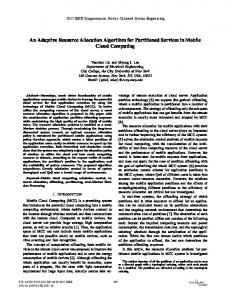
about one second, as seen from Table 2. In Figure 3 and Figure 4, we give the speed-up ratio computed using the running times as

1 30 τ HBBA i , ∑ 30 i =1 τ BBA i where τ BBA i denotes the running time of the Pure BBA and τ HBBA i is the running time of the BBA-phase (Step 2) of the HBBA for the problem number i in a particular series. Note that we used 30 instances in each series, so i=1,2,…,30. The confidence intervals correspond to 95% level. The results for other series have the same sort of behavior. For series GN_m, the speed-up factor is always present on these problems and it approaches the ratio 0.6 approximately (see Figure 3). For series W8_m, with the growth of problem size, the acceleration becomes more significant, approaching 0.06 (see Figure 4).

[Insert Figure 3 about here] [Insert Figure 4 about here]

4.2 Known knapsack-type tests

Many publications focus on knapsack formulations of buffer space allocation problem. Therefore, we also tested our algorithms on two series of 5-machine knapsack-type problems vp6.3 - vp6.10 and vp7.3 - vp7.10 which were suggested by Vouros and Papadopoulos (1998). In their paper, the overall amount of buffer space was limited

20

from above by the value given in the problem index (i.e. for k = 3, 4, …, 10, the set of admissible solutions for vp6.k and vp7.k is restricted by the condition B(H) ≤ k). The maximization criterion is the output rate V(H).

In order to take into account the knapsack-type constraint in our case, we have defined

ϕ(H) combining the output rate with a linear penalty: ϕ(H)=V(H)-10000×max{0,B(H)k}. For all of these test examples, we set the buffer acquisition cost J(H) equal to B(H) and the amortization time Tam=1, so the revenue is R(V(H)) = V(H). The parameters of machines in series vp6.3 - vp6.10 were the following: µ1= µ2= µ3= µ4= µ5= 0.5, λ1= 0.1, λ2= 0.2, λ3= 0.25, λ4= 0.3, λ5= 0.35, u1= u2= u3= u4= u5= 1. Here we set the production rates u1, u2, …, u5 equal to the corresponding mean production rates in (Vouros and Papadopoulos, 1998). Similarly we assign the following parameters of machines in series vp7.3 - vp7.10: µ1= µ2= µ3= µ4= µ5= 0.5, λ1= λ2= λ3= λ4= λ5= 0.05, u1= 1, u2= 1.1, u3= 1.2, u4= 1.3, and u5= 1.4.

In Table 3, we show the solutions for vp6.3-vp6.10 and vp7.3 - vp7.10 obtained by the Pure BBA (column H), their goal function values (column ϕ), and the corresponding running time. [Insert Table 3 about here]

Note that the BBA time for considered knapsack-type problems is very short (