The Adaptable Buffer Algorithm for High Quantile Estimation in

The Adaptable Buffer Algorithm for High Quantile Estimation in Non-Stationary Data Streams Ognjen Arandjelovi´c† , Duc-Son Pham‡ , and Svetha Venkatesh†

arXiv:1504.05302v1 [cs.CV] 21 Apr 2015

†

Centre for Pattern Recognition & Data Analytics Deakin University Geelong VIC 3216 Australia

Abstract—The need to estimate a particular quantile of a distribution is an important problem which frequently arises in many computer vision and signal processing applications. For example, our work was motivated by the requirements of many semi-automatic surveillance analytics systems which detect abnormalities in close-circuit television (CCTV) footage using statistical models of low-level motion features. In this paper we specifically address the problem of estimating the running quantile of a data stream with non-stationary stochasticity when the memory for storing observations is limited. We make several major contributions: (i) we derive an important theoretical result which shows that the change in the quantile of a stream is constrained regardless of the stochastic properties of data, (ii) we describe a set of high-level design goals for an effective estimation algorithm that emerge as a consequence of our theoretical findings, (iii) we introduce a novel algorithm which implements the aforementioned design goals by retaining a sample of data values in a manner adaptive to changes in the distribution of data and progressively narrowing down its focus in the periods of quasi-stationary stochasticity, and (iv) we present a comprehensive evaluation of the proposed algorithm and compare it with the existing methods in the literature on both synthetic data sets and three large ‘real-world’ streams acquired in the course of operation of an existing commercial surveillance system. Our findings convincingly demonstrate that the proposed method is highly successful and vastly outperforms the existing alternatives, especially when the target quantile is high valued and the available buffer capacity severely limited.

I. I NTRODUCTION Quantile estimation is of pervasive importance across a variety of signal processing applications. It is used extensively in data mining, simulation modelling [14], database maintenance, risk management in finance [1], [26], and the analysis of computer network latencies [7], [8], amongst others. A particularly challenging form of the quantile estimation problem arises when the desired quantile is high-valued (close to unity) and when data needs to be processed as a stream, with limited memory capacity. An illustrative practical example of when this is the case is encountered in CCTVbased surveillance systems [6]. In summary, as various types of low-level observations related to events in the scene of interest arrive in real-time, quantiles of the corresponding statistics for time windows of different durations are needed in order

‡

Department of Computing Curtin University Perth WA 6845 Australia

to distinguish ‘normal’ (common) events from those which are in some sense unusual and thus require human attention. The amount of incoming data is extraordinarily large and the capabilities of the available hardware highly limited both in terms of storage capacity and processing power. A. Previous work Unsurprisingly, the problem of estimating a quantile of a set has received considerable attention, much of it in the realm of theoretical research. In particular, a substantial amount of work has focused on the study of asymptotic computational complexity of quantile estimation algorithms [11], [20]. An important result emerging from this corpus of work is the proof by Munro and Paterson [20] that the working memory requirement of any algorithm that determines the median of a set by making at most p sequential passes through the input is Ω(n1/p ) (i.e. asymptotically growing at least as fast as n1/p ). This implies that the exact computation of a quantile requires Ω(n) working memory. Therefore a single-pass algorithm, required to process streaming data, will necessarily produce an estimate and not be able to guarantee the exactness of its result. Most of the quantile estimation algorithms developed for use in practice are not single-pass algorithms and thus cannot be applied to streaming data [12]. On the other hand, many single-pass approaches focus on the exact computation of the quantile and therefore, as explained previously, demand the O(n) storage space which is clearly an unfeasible proposition in the context we consider in the present paper; this includes the work by Greenwald and Khanna [10] who described an O(n) method efficient in the sense that it attains the asymptotic minimum in the space requirement as a function of the permissible error in the desired quantile estimate. Amongst the few methods described in the literature which satisfy the practical constraints of interest in the present paper are the histogrambased method of Schmeiser and Deutsch [25] (with a similar approach described by McDermott et al. [19]), and the P 2 algorithm of Jain and Chlamtac [14]. Schmeiser and Deutsch maintain a preset number of bins, scaling their boundaries to cover the entire data range as needed and keeping them

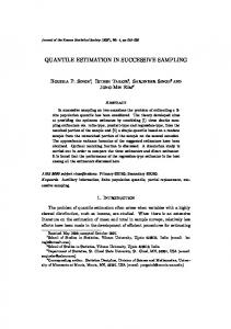
evaluation of different methods in Section III), in Figure 1. In particular, the top plot in this figure shows the variation of the ground-truth 0.95-quantile which corresponds to the data stream shown in the bottom plot. Notice that the quantile exhibits little variation over the course of approximately the first 75% of the duration of the time window (the first 190,000 data points). This corresponds to a period of little activity in the video from which the data is extracted (see Section III-A for a detailed explanation). Then, the value of the quantile increases rapidly for over an order of magnitude – this is caused by a sudden burst of activity in the surveillance video and the corresponding change in the statistical behaviour of the data.

11

6

4 3 2 1 0

II. P ROPOSED ALGORITHM

1

1.5

2 Datum index

A. Quantiles Let p be the probability density function of a real-valued random variable X. Then the q-quantile vq of p is defined as [15]: Z vq p(x) dx = q. (1) −∞

Similarly, the q-quantile of a finite set D can be defined as:

2.5 5

x 10

11

15

Datum value

We begin by a formalization of the notion of a quantile, follow by a derivation of the key results underlying our contribution, and finally a describe the proposed algorithm.

|{x : x ∈ D and x ≤ vq }| ≤ q × |D|.

x 10

5 Quantile estimate

equidistant. Jain and Chlamtac attempt to maintain a small set of ad hoc selected key points of the data distribution, updating their values using quadratic interpolation as new data arrives. Various random sample methods, such as that described by Vitter [27], and Cormode and Muthukrishnan [9], use different sampling strategies to fill the available buffer with random data points from the stream, and estimate the quantile using the distribution of values in the buffer. Lastly, the recently proposed algorithm of Arandjelovi´c et al. [3] employs an adaptable quasi-maximum entropy histogram; their approach is discussed further in Section II-B. In addition to the ad hoc elements of the existing algorithms for quantile estimation on streaming data, which itself is a sufficient cause for concern when the algorithms need to be deployed in applications which demand high robustness and well understood failure modes, it is also important to recognize that an implicit assumption underlying these approaches (with the exception of the algorithm of Arandjelovi´c et al. [3]; see Section II-B) is that the data is governed by a stationary stochastic process. The assumption is often invalidated in realworld applications.

x 10

10

5

0

1

1.5

2 Datum index

2.5 5

x 10

Fig. 1. An example of a rapid change in the value of a quantile (specifically the 0.95-quantile in this case) on a real-world data stream used for surveillance video analysis (see Section III-A).

(2)

In other words, the q-quantile is the smallest value below which q fraction of the total values in a set lie. The concept of a quantile is thus intimately related to the tail behaviour of a distribution. B. Challenges of non-stochasticity In this work our aim is to develop a method for quantile estimation applicable not only to streams which exhibit stationary stochasticity but also to the all-encompassing set of streams which includes those with non-stationary data. It is a straightforward consequence of potential non-stationarity that at no point in time can it be assumed that the historical distribution of data values is representative of the future distribution of the stream data. This is true regardless of how much historical data has been seen. Thus, the value of a particular quantile can change greatly and rapidly, in either direction (i.e. increase or decrease). This is illustrated on an example, extracted from a real-world data set used for surveillance video analysis (the full data corpus is used for comprehensive

It may appear to be the case that to be able to adapt to such unpredictable variability in input it is necessary to maintain an approximation of the entire distribution of historical data. Indeed, this is argued in a recent work which introduced the Data-Aligned Maximum Entropy Histogram algorithm for quantile estimation from streams [3]. The method employs a histogram of a fixed length, determined by the available working memory, which adjusts bin boundary values in a manner which maximizes the entropy of the corresponding estimate of the historical data distribution. Although it is true that the change in the value of a specific quantile may be of an arbitrary large magnitude, in this paper we show that its specific value in a particular stream is nevertheless constrained. Succinctly put, this is a consequence of the fact that although the stream data may be considered as being drawn from a continuous probability density function (which may change with time) the information available to our algorithm inherently comprises discrete quanta: individual data points.

C. Constraints: key theoretical results Consider a stream of values x1 , x2 , . . . , xn . For the time being let us assume that there are no repeated values in the stream i.e. ∀i, j. xi = xj =⇒ i = j. Then there is an indexing function f (. . .) such that xfn (1) < xfn (2) < . . . < xfn (n) . Let xq(n) = xf (k) be the current estimate of a particular quantile q of interest. Consider ∆k, the change in k that the arrival of a new datum xn+1 effects. By definition given in Equation 2: ∆k =b(1 − q) × (n + 1)c − b(1 − q) × nc.

(3)

Exploiting simple properties of the flood function then leads to the following series of inequalities and an upper bound on the value of ∆k: ∆k =b(1 − q) × (n + 1)c − b(1 − q) × nc

(4)

≤(1 − q) × (n + 1) − b(1 − q) × nc

(5)

=(1 − q) × n − b(1 − q) × nc + (1 − q)

(6)

b1 , the new datum xn+1 is inserted into the buffer and the largest value in the buffer, bm , discarded. The former case reinforces the central positioning of the current quantile estimate, while the latter acts so as to decrease the spread of values within the buffer. The auxiliary count corresponding to the newly inserted datum is initialized by linearly interpolating between the counts of buffer values between which the datum is inserted. Auxiliary counts corresponding to lower valued buffer elements are left unchanged while those corresponding to higher valued elements are increased by one. Similarly, if the new datum is greater than the current quantile estimate, i.e. xn+1 > bk , and either k > bm/2c or xn+1 < bm , the new datum xn+1 is inserted into the buffer and the smallest value in the buffer, b1 , discarded. III. E VALUATION We now turn our attention to the evaluation of the proposed algorithm. In particular, to assess its effectiveness and compare it with the algorithms described in the literature, in this section we report its performance on three large ‘real-world’ data streams. A. Real-world surveillance data Computer-assisted video surveillance data analysis is of major commercial and law enforcement interest. On a broad

scale, systems currently available on the market can be grouped into two categories in terms of their approach. The first group focuses on a relatively small, predefined and well understood subset of events or behaviours of interest such as the detection of unattended baggage, violent behaviour, etc [24], [16]. The narrow focus of these systems prohibits their applicability in less constrained environments in which a more general capability is required. These approaches tend to be computationally expensive and error prone, often requiring fine tuning by skilled technicians. This is not practical in many circumstances, for example when hundreds of cameras need to be deployed as often the case with CCTV systems operated by municipal authorities. The second group of systems approaches the problem of detecting suspicious events at a semantically lower level [13], [22], [18], [2], [4]. Their central paradigm is that an unusual behaviour at a high semantic level will be associated with statistically unusual patterns (also ‘behaviour’ in a sense) at a low semantic level – the level of elementary image/video features. Thus methods of this group detect events of interest by learning the scope of normal variability of low-level patterns and alerting to anything that does not conform to this model of what is expected in a scene, without ‘understanding’ or interpreting the nature of the event itself. These methods uniformly start with the same procedure for feature extraction. As video data is acquired, firstly a dense optical flow field is computed using the wellknown method of Lucas and Kanade [17]. Then, to reduce the amount of data that needs to be processed, stored, or transmitted, a thresholding operation is performed. This results in a sparse optical flow field whereby only those flow vectors whose magnitude exceeds a certain value are retained; nonmaximum suppression is applied here as well [23]. Normal variability within a scene and subsequent novelty detection are achieved using various statistics computed over this data. The data streams, shown partially in Figure 2, correspond to the values of such statistics (their exact meaning is proprietary and has not been made known fully to the authors of the present paper either). Observe the non-stationary nature of the streams which is evident both on the long and short time scales (magnifications are shown for additional clarity and insight). Table I provides a summary of some of the key features of the three data sets acquired in the described manner and used for the evaluation in this paper.

TABLE I K EY STATISTICS OF THE THREE REAL - WORLD DATA SETS USED IN OUR EVALUATION .

Data set

Data points

Stream 1

555, 022

Stream 2

10, 424, 756

Stream 3

1, 489, 618

Mean value 10

7.81 × 10 2.25

1.51 × 10

Standard deviation 1.65 × 1011 15.92

5

2.66 × 106

B. Results We compared the performances of our algorithm and the four alternatives from the literature described in Section I-A: (i) the P 2 algorithm of Jain and Chlamtac [14], (ii) the random sample based algorithm of Vitter [27], (iii) the uniform adjustable histogram of Schmeiser and Deutsch [25], and (iv) the data-aligned maximal entropy histogram of Arandjelovi´c et al. [3], [5]. A representative summary of results is shown in Table II. It can be readily observed that our method and the method of Arandjelovi´c et al. significantly outperformed other approaches. The P 2 and equispaced histogram based algorithms performed worst, often producing highly inaccurate estimates. The random sample algorithm of Vitter performed relatively well but still substantially worse than the top two methods. It is interesting to note that the data-aligned maximal entropy histogram of Arandjelovi´c et al. outperformed the proposed method. At first we found this highly surprising given that this algorithm approximates the entire distribution of historical data whereas ours, by design, narrows its focus to the more relevant part of the distribution. We hypothesized that the reason behind this is that the quantile we sought to estimate was insufficiently challenging (not close enough to 1, relative to buffer size). Specifically, our hypothesis stems from the observation that some information is lost by interpolation every time a new datum is added to our buffer. While interpolation is also employed by Arandjelovi´c et al., when the target quantile is not particularly challenging relative to the buffer size, the number of interpolations performed by the simple data-aligned maximal entropy histogram is lower and its underlying model sufficiently flexible to produce an accurate estimate. Consequently, we hypothesized that the advantages of our method would only be fully exhibited for higher quantiles (needed in applications such as customer wallet estimation [21]) and we sought to investigate that next. In the second set of experiments we compared our method with the data-aligned maximal entropy histogram of Arandjelovi´c et al. using a series of progressively challenging target quantiles. A summary of the results is shown in Table III. It is readily apparent that this set of results fully supports our hypothesis. While our algorithm showed an improvement in performance as the value of the target quantile was increased, the opposite was true for the data-aligned maximal entropy histogram which performed progressively worse. Data set 3 again proved to be the most challenging one, the data-aligned maximal entropy histogram producing grossly inaccurate estimates for quantile values of over 0.99. For example, on stream 3 for the target quantile of 0.999 the data-aligned maximal entropy histogram achieved the average relative L1 error of 368.6%, while the proposed algorithm showed remarkable accuracy and the error of 1.6%. The same observations can be made by considering the absolute L∞ error i.e. the greatest error in the running quantile estimates, which were respectively 2.35e7 and 3.35e6 – a difference of approximately an order of magnitude. Table III also includes a column (right-most) showing the

TABLE II C OMPARATIVE EXPERIMENTAL RESULTS FOR 0.95- QUANTILE .

Stream 1 Method

Bins

Stream 2

Stream 3

Relative

Absolute

Relative

Absolute

Relative

Absolute

L1 error

L∞ error

L1 error

L∞ error

L1 error

L∞ error

Targeted adaptable

500

2.1%

1.00e11

4.7%

24.20

5.2%

4.8e5

sample (proposed)

100

1.6%

1.07e11

9.2%

54.73

3.6%

2.89e5

Data-aligned max.

500

1.2%

3.11e10

0.0%

2.04

0.1%

8.11e4

entropy histogram [3]

100

9.6%

2.06e11

0.0%

1.91

2.6%

3.33e5

P 2 algorithm [14]

n/a

15.7%

2.77e11

3.1%

93.04

84.2%

1.55e6

Random sample [27]

500

4.6%

1.98e11

0.7%

38.00

10.4%

5.95e5

Equispaced histogram [25]

500

87.1%

1.07e12

0.1%

80.29

675.1%

4.39e7

Stream 3

Stream 2

Stream 1

Proposed method Quantile

Data-aligned histogram

Max value to quantile ratio

Data set

TABLE III C OMPARISON OF THE TOP TWO ALGORITHMS FOR HIGH - VALUE QUANTILES USING 100 BINS .

Relative

Absolute

Relative

Absolute

L1 error

L∞ error

L1 error

L∞ error

0.9500

1.6%

1.07e11

9.6%

2.06e11

15.8

0.9900

1.2%

9.59e10

27.9%

5.69e11

5.9

0.9950

2.1%

9.27e10

58.8%

8.48e11

4.2

0.9990

0.7%

9.80e10

48.0%

9.47e11

2.1

0.9995

0.3%

2.69e10

36.8%

8.72e11

1.5

0.9500

9.2%

54.73

0.0%

1.91

30.1

0.9900

2.4%

26.31

0.3%

2.45

2.5

0.9950

0.3%

6.21

0.2%

4.59

1.8

0.9990

0.2%

16.05

0.4%

30.29

1.4

0.9995

0.2%

20.17

2.0%

34.44

1.3

0.9500

3.6%

2.89e5

2.6%

3.33e5

520.3

0.9900

1.2%

3.32e6

2.4%

3.25e5

122.7

0.9950

1.8%

1.40e6

480.5%

1.63e8

60.9

0.9990

1.6%

3.35e6

368.6%

2.35e7

11.7

0.9995

4.2%

1.30e7

364.2%

2.34e8

7.2

300

Datum value

250

12

3

x 10

Datum value

2.5

200 150 100 50

2

0

0

2

4

6 Datum index

1.5

8

10

12 6

x 10

250

1

200

0.5 0

150 100

0

1

2

3 Datum index

4

5

6 5

x 10

50 0

0

100

200

300

400

(a) Data stream 1

500

600

700

800

900

1000

(b) Data stream 2 8

3

x 10

2.5 Datum value

6500 6000 5500 5000 4500

2 1.5 1

4000 3500

0

100

200

300

400

500

600

700

800

900

0.5

1000

0

0

5

10

15

Datum index

5

x 10

(c) Data stream 3

Fig. 2.

The three large ‘real-world’ data streams used in our evaluation.

6

xz10

50

1.5

Value

Buffer size: 100 Buffer size: 12

Groundztruth Bufferzsize:z12 Bufferzsize:z25 Bufferzsize:z100

40 Location in buffer

2

1

0.5

30

20

10 0

0

1

2

3

4 5 Datumzindex

6

7

8

0

9 5

xz10

Fig. 3. An example running ground truth of the target quantile (q = 0.95) and the estimates of our algorithm for different bin sizes on data stream 3. It is remarkable to observe that our method achieved a consistently highly accurate estimate even when the available buffer capacity was severely restricted (down to only 12 bins).

ratio of the maximal stream value and the ground truth for the target quantile. We sought to examine if a particularly high ratio predicts poor performance of the data-aligned maximal entropy histogram, which may be expected given that throughout its operation the algorithm approximates the entire distribution of historical data. We found this not to be the case which can be explained by the allocation of bin ranges according to the maximum entropy principle and the alignment of the bin boundaries with data; please see the original publication for a detailed description of the method [3]. Lastly, we sought to analyse the performance of the proposed method in additional detail. Figure 3 shows on an example the running ground truth of the target quantile (q = 0.95) and the estimates of our algorithm for different bin sizes on the most challenging data stream 3. It is remarkable

0

5 10 Quantile ceiling location (relative to buffer centre)

15 5

x 10

Fig. 4. Our algorithm is highly successful in achieving one of the key ideas behind the method, that of adapting the data sample retained in the buffer so as to maintain the position of the current quantile estimate in the buffer as close to its centre as possible (see Section II-C). Both in the case of a buffer with the capacity of 100 and 12 (the results for only two buffer sizes are shown to reduce clutter), the central positioning of the quantile estimate is maintained very tightly throughout the processing of the stream.

to observe that our method consistently achieved a highly accurate estimate even when the available buffer capacity was severely restricted (to 12 bins). In Figure 4 the same example run was used to illustrate the success of our algorithm in achieving one of the key ideas behind the method, that of adapting the data sample retained in the buffer so as to maintain the position of the current quantile estimate in the buffer as close to its centre as possible (see Section II-C). As the plot clearly shows, both in the case of a buffer with the capacity of 100 and 12 (the results for only two buffer sizes are shown to reduce clutter), the central positioning of the quantile estimate is maintained very tightly throughout the processing of the stream. Similarly, the success of our

11

x(10

0.95−quantile(ground(truth Cumulative(data(maximum Buffer(spred((@(size(12)

2.5 Relative L1 error (%)

Datum(value

2.5 2 1.5 1

1.4

2 1.2 1.5 1 1 0.8

0.5

0.5 0

x 10 1.6

3

0

5

10

15

Datum(index

5

x(10

Fig. 5. The success of our algorithm in achieving tight sampling of the data distribution around the target quantile – unlike the random sample based algorithm of Vitter [27] or the uniform adjustable histogram of Schmeiser and Deutsch [25] which retain a sample from a wide range of values, our method utilizes the available memory efficiently by focusing on a narrow spread of values around the current quantile estimate. While the spread of values in the buffer experiences intermittent and transient increases when there is a burst of high valued data points in preparation for a potentially large quantile change, thereafter it quickly adapts to the correct part of the distribution.

Absolute L∞ error

8

3

0

100

200

300

400 Buffer size

500

600

700

0.6 800

Fig. 7. The variation in the accuracy of our algorithm’s estimate with the buffer size on data stream 3. Unlike any of the existing algorithms, our method exhibits very gradual and graceful degradation in performance, and still achieves remarkable accuracy even with a severely restricted buffer capacity.

IV. S UMMARY AND CONCLUSIONS algorithm in achieving tight sampling of the data distribution around the target quantile is illustrated in the plot in Figure 5. This plot shows that unlike the random sample based algorithm of Vitter [27] or the uniform adjustable histogram of Schmeiser and Deutsch [25] which retain a sample from a wide range of values, our method utilizes the available memory efficiently by focusing on a narrow spread of values around the current quantile estimate. Note that the spread of values in the buffer experiences intermittent and transient increases when there is a burst of high valued data points in preparation for a potentially large quantile change, but thereafter quickly adapts to the correct part of the distribution. The variation in the mean buffer spread with the buffer size and target quantile is shown in Figure 6. Lastly, the variation in the accuracy of our algorithm’s estimate with the buffer size is analysed in Figure 7. Unlike any of the existing algorithms, our method exhibits very gradual and graceful degradation in performance, and still achieves remarkable accuracy even with a severely restricted buffer capacity.

In this paper we described a novel algorithm for the estimation of a quantile of a data stream when the available working memory is limited (constant), prohibiting the storage of all historical data. This problem is ubiquitous in computer vision and signal processing, and has been addressed by a number of researchers in the past. We showed that a major shortcoming of the existing methods lies in their usually implicit assumption that the data is being generated by a stationary process. This assumption is invalidated in most practical applications, as we illustrated using real-world data. Evaluated on three large data streams extracted from CCTV footage, our algorithm was vastly superior in comparison with the existing alternatives. The highly non-stationary nature of the data was shown to cause major problems to previous methods, often leading to grossly inaccurate quantile estimates; in contrast, our method was virtually unaffected by it. What is more, our experiments demonstrate that the superior performance of our algorithm can be maintained effectively while drastically reducing the working memory size in comparison with the methods from the literature.

0.05

R EFERENCES

Mean buffer spread

0.04

0.03

0.995−quantile 0.99−quantile 0.95−quantile

0.02

0.01

0 10

20

30

40

50 60 Buffer size

70

80

90

100

Fig. 6. The variation in the mean buffer spread with the buffer size and target quantile on data stream 3.

[1] R. Adler, R. Feldman, and M. Taqqu, editors. A Practical Guide to Heavy Tails. Statistical Techniques and Applications. Birkh¨auser, 1998. [2] O. Arandjelovi´c. Contextually learnt detection of unusual motion-based behaviour in crowded public spaces. In Proc. International Symposium on Computer and Information Sciences, pages 403–410, 2011. [3] O. Arandjelovi´c, D. Pham, and S. Venkatesh. Stream quantiles via maximal entropy histograms. In Proc. International Conference on Neural Information Processing, II:327–334, 2014. [4] O. Arandjelovi´c, D. Pham, and S. Venkatesh. CCTV scene perspective distortion estimation from low-level motion features. IEEE Transactions on Circuits and Systems for Video Technology, 2015. DOI: 10.1109/TCSVT.2015.2424055.

[5] O. Arandjelovi´c, D. Pham, and S. Venkatesh. Two maximum entropy based algorithms for running quantile estimation in non-stationary data streams. IEEE Transactions on Circuits and Systems for Video Technology, 25, 2015. DOI: 10.1109/TCSVT.2014.2376137. [6] O. Arandjelovi´c, D. Pham, and S. Venkatesh. Viewpoint distortion compensation in practical surveillance systems. In Proc. International Conference on Multimedia and Expo, 2015. [7] C. Buragohain and S. Suri. Encyclopedia of Database Systems, chapter Quantiles on Streams., pages 2235–2240. 2009. [8] G. Cormode, T. Johnson, F. Korn, S. Muthukrishnany, O. Spatscheck, and D. Srivastava. Holistic UDAFs at streaming speeds. In Proc. ACM SIGMOD International Conference on Management of Data, pages 35– 46, 2004. [9] G. Cormode and S. Muthukrishnany. An improved data stream summary: the count-min sketch and its applications. Journal of Algorithms, 55(1):58–75, 2005. [10] M. Greenwald and S. Khanna. Space-efficient online computation of quantile summaries. ACM SIGMOD Record, 30(2):58–66, 2001. [11] S. Guha and A. McGregor. Stream order and order statistics: Quantile estimation in random-order streams. SIAM Journal on Computing,, 38(5):2044–2059, 2009. [12] A. P. Gurajada and J. Srivastava. Equidepth partitioning of a data set based on finding its medians. Technical report TR 90-24, Computer Science Department, University of Minnesota, 1990. [13] iCetana. iMotionFocus. http:// www.icetana.com/ , Accessed May 2014. [14] R. Jain and I. Chlamtac. The P 2 algorithm for dynamic calculation of quantiles and histograms without storing observations. Communications of the ACM, 28(10):1076–1085, 1985. [15] J. F. Kenney and E. S. Keeping. Mathematics of Statistics., volume 1, chapter Quantiles., pages 37–38. Van Nostrand, 3rd edition, 1962. [16] G. Lavee, L. Khan, and B. Thuraisingham. A framework for a video analysis tool for suspicious event detection. Multimedia Tools and Applications, 35(1):109–123, 2007. [17] B. Lucas and T. Kanade. An iterative image registration technique with an application to stereo vision. In Proc. International Joint Conference on Artificial Intelligence (IJCAI), I:674–679, 1981. [18] R. Martin and O. Arandjelovi´c. Multiple-object tracking in cluttered and crowded public spaces. In Proc. International Symposium on Visual Computing, 3:89–98, 2010. [19] J. P. McDermott, G. J. Babu, J. C. Liechty, and D. K. J. Lin. Data skeletons: simultaneous estimation of multiple quantiles for massive streaming datasets with applications to density estimation. Bayesian Analysis, 17:311–321, 2007. [20] J. I. Munro and M. Paterson. Selection and sorting with limited storage. Theoretical Computer Science, 12:315–323, 1980. [21] C. Perlich, S. Rosset, R. D. Lawrence, and B. Zadrozny. High-quantile modeling for customer wallet estimation and other applications. In Proc. ACM SIGKDD International Conference on Knowledge Discovery and Data (KDD), pages 977–985, 2007. [22] D. Pham, O. Arandjelovi´c, and S. Venkatesh. Detection of dynamic background due to swaying movements from motion features. IEEE Transactions on Image Processing, 24(1):332–344, 2015. [23] T. Q. Pham. Non-maximum suppression using fewer than two comparisons per pixel. In Proc. Advanced Concepts for Intelligent Vision Systems (ACIVS), pages 438–451, 2010. [24] Philips Electronics N.V. A surveillance system with suspicious behaviour detection. Patent EP1459272A1, 2004. [25] B. W. Schmeiser and S. J. Deutsch. Quantile estimation from grouped data: The cell midpoint. Communications in Statistics: Simulation and Computation, B6(3):221–234, 1977. [26] N. Sgouropoulos, Q. Yao, and C. Yastremiz. Matching quantiles

estimation. Technical report, London School of Economics, 2013. [27] J. S. Vitter. Random sampling with a reservoir. ACM Transactions on Mathematical Software, 11(1):37–57, 1985.