HD-CNN: Hierarchical Deep Convolutional Neural Networks for ... - HKU

HD-CNN: Hierarchical Deep Convolutional Neural Networks for Large Scale Visual Recognition Zhicheng Yan† , Hao Zhang‡ , Robinson Piramuthu∗ , Vignesh Jagadeesh∗ , Dennis DeCoste∗ , Wei Di∗ , Yizhou Yu?† † University of Illinois at Urbana-Champaign, ‡ Carnegie Mellon University ∗ eBay Research Lab, ? The University of Hong Kong

Abstract In image classification, visual separability between different object categories is highly uneven, and some categories are more difficult to distinguish than others. Such difficult categories demand more dedicated classifiers. However, existing deep convolutional neural networks (CNN) are trained as flat N-way classifiers, and few efforts have been made to leverage the hierarchical structure of categories. In this paper, we introduce hierarchical deep CNNs (HD-CNNs) by embedding deep CNNs into a two-level category hierarchy. An HD-CNN separates easy classes using a coarse category classifier while distinguishing difficult classes using fine category classifiers. During HDCNN training, component-wise pretraining is followed by global fine-tuning with a multinomial logistic loss regularized by a coarse category consistency term. In addition, conditional executions of fine category classifiers and layer parameter compression make HD-CNNs scalable for largescale visual recognition. We achieve state-of-the-art results on both CIFAR100 and large-scale ImageNet 1000-class benchmark datasets. In our experiments, we build up three different two-level HD-CNNs, and they lower the top-1 error of the standard CNNs by 2.65%, 3.1%, and 1.1%.

1. Introduction Deep CNNs are well suited for large-scale supervised visual recognition tasks because of their highly scalable training algorithm. It only needs to cache a small chunk of the potentially huge volume of training data during sequential scans. One of the complications that arises in large datasets with a large number of categories is that the visual separability of object categories is highly uneven. Some categories are much harder to distinguish than others. Take the categories in CIFAR100 as an example. It is easy to tell an Apple from a Bus, but harder to tell an Apple from an Orange. In fact, both Apples and Oranges belong to the same

coarse category fruit and vegetables, while Buses belong to another coarse category, vehicles 1, as defined within CIFAR100. Nonetheless, most deep CNN models nowadays are flat N-way classifiers, which share a set of fully connected layers. This makes us wonder whether such a flat structure is adequate for distinguishing all the difficult categories. A very natural and intuitive alternative organizes classifiers in a hierarchical manner according to the divideand-conquer strategy. Although hierarchical classification has been proven effective for conventional linear classifiers [38, 8, 37, 22], few attempts have been made to exploit category hierarchies [3, 29] in deep CNN models. Since deep CNN models are large models themselves, organizing them hierarchically imposes the following challenges. First, instead of a handcrafted category hierarchy, how can we learn such a category hierarchy from the training data itself so that cascaded inferences in a hierarchical classifier will not degrade the overall accuracy while dedicated fine category classifiers exist for hard-to-distinguish categories? Second, a hierarchical CNN classifier consists of multiple CNN models at different levels. How can we leverage the commonalities among these models and effectively train them all? Third, it would also be slower and more memory consuming to run a hierarchical CNN classifier on a novel testing image. How can we alleviate such limitations? In this paper, we propose a generic and principled hierarchical architecture, Hierarchical Deep Convolutional Neural Network (HD-CNN), that decomposes an image classification task into two steps. First, easy classes are separated by a coarse category CNN classifier. Second, challenging classes are routed downstream to fine category classifiers. HD-CNN is modular and is built upon a building block CNN, which can be chosen to be any of the stateof-the-art single CNN. An HD-CNN follows the coarse-tofine classification paradigm and probabilistically integrates predictions from fine category classifiers. We show that HD-CNN can achieve lower error than the corresponding building block CNN, at the cost of a manageable increase

Root

Coarse  component independent  layers  B

Fine  component   independent  layers  F1 . . .

Coarse category 2: {toy terrier, greyhound, whippet, basenji, … } .   .   .  

Image

Coarse category K: {mink, cougar, bear, fox squirrel, otter, … }

Shared   layers

(a)

low-­level  features

Fine  component   independent  layers  FK

fine   prediction  1

fine   prediction  K

Probabilistic  a veraging  layer

coarse  p rediction

Coarse category 1: {white shark, numbfish, hammerhead, stingray, … }

final   prediction

(b)

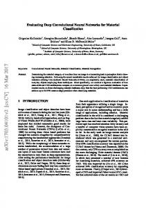
Figure 1: (a) A two-level category hierarchy where the classes are taken from ImageNet 1000-class dataset. (b) Hierarchical Deep Convolutional Neural Network (HD-CNN) architecture. in memory footprint and classification time. In summary, this paper has the following contributions. First, we introduce HD-CNN, a novel hierarchical architecture for image classification. Second, we develop a scheme for learning the two-level organization of coarse and fine categories, and demonstrate that various components of an HD-CNN can be independently pretrained. The complete HD-CNN is further fine-tuned using a multinomial logistic loss regularized by a coarse category consistency term. Third, we make the HD-CNN scalable by compressing the layer parameters and conditionally executing the fine category classifiers. We demonstrate state-of-the-art performance on both CIFAR100 and ImageNet.

2. Related Work Our work is inspired by rapid progress in CNN design and integration of category hierarchy with linear classifiers. The main novelty of our method is the scalable HD-CNN architecture that integrates a category hierarchy with deep CNNs.

2.1. Convolutional Neural Networks CNN-based models hold state-of-the-art performance in various computer vision tasks, including image classifcation [18], object detection [10, 13], and image parsing [7]. Recently, there has been considerable interest in enhancing CNN components, including pooling layers [36], activation units [11, 28], and nonlinear layers [21]. These enhancements either improve CNN training [36], or expand the network learning capacity. This work boosts CNN performance from an orthogonal angle and does not redesign a specific part within any existing CNN model. Instead, we design a novel generic hierarchical architecture that uses an existing CNN model as a building block. We embed multiple building blocks into a larger hierarchical deep CNN.

ated given a testing image scales sublinearly in the number of classes [2, 9]. The hierarchy can be either predefined [23, 33, 16] or learned by top-down and bottom-up approaches [25, 12, 24, 20, 1, 6, 27]. In [5], the predefined category hierarchy of the ImageNet dataset is utilized to achieve trade-offs between classification accuracy and specificity. In [22], a hierarchical label tree is constructed to probabilistically combine predictions from leaf nodes. Such a hierarchical classifier achieves significant speedup at the cost of certain accuracy loss. One of the earliest attempts to introduce a category hierarchy in CNN-based methods is reported in [29], but their main goal was transferring knowledge between classes to improve the results for classes with insufficient training examples. In [3], various label relations were encoded in a hierarchy. Improved accuracy is achieved only when a subset of training images is relabeled with internal nodes in the hierarchical class tree. They are not able to improve accuracy in the original setting where all training images are labeled with leaf nodes. In [34], a hierarchy of CNNs is introduced, but they experimented with only two coarse categories, mainly due to scalability constraints. HD-CNN exploits the category hierarchy in a novel way in that we embed deep CNNs into the hierarchy in a scalable manner and achieve superior classification results over standard CNN.

3. Overview of HD-CNN 3.1. Notations The dataset consists of a set of pairs {xi , yi }, where xi is an image and yi its category label. C denotes the number of fine categories, which will be automatically grouped c K into K coarse categories. {Sjf }C j=1 and {Sk }k=1 are partitions of image indices based on fine and coarse categories. Superscripts f and c denote fine and coarse categories.

2.2. Category Hierarchy for Visual Recognition In visual recognition, there is a vast literature exploiting category hierarchical structures [32]. For classification with a large number of classes using linear classifiers, a common strategy is to build a hierarchy or taxonomy of classifiers so that the number of classifiers evalu-

3.2. HD-CNN Architecture HD-CNN is designed to mimic the structure of category hierarchy, where fine categories are grouped into coarse categories, as in Fig 1(a). It performs end-to-end classification, as illustrated in Fig 1(b). It mainly comprises four parts: (i)

shared layers, (ii) a single component B to handle coarse categories, (iii) multiple components {Fk }K k=1 (one for each group) for fine classification, and (iv) a single probabilistic averaging layer. Shared layers (left of Fig 1 (b)) receive raw image pixels as input and extract low-level features. The configuration of shared layers is set to be the same as the preceding layers in the building block CNN. On the top of Fig 1(b) are independent layers of coarse category component B, which reuses the configuration of rear layers from the building block CNN and produces an f C intermediate fine prediction {Bij }j=1 for an image xi . To produce a coarse category prediction {Bik }K k=1 , we append a fine-to-coarse aggregation layer (not shown in Fig 1(b)), which reduces fine predictions into coarse using a mapping P : [1, C] 7→ [1, K]. The coarse category probabilities serve two purposes. First, they are used as weights for combining the predictions made by fine category components {Fk }K k=1 . Second, when thresholded, they enable conditional execution of fine category components whose corresponding coarse probabilities are sufficiently large. In the bottom right of Fig 1 (b) are independent layers of a set of fine category classifiers {Fk }K k=1 , each of which makes fine category predictions. As each fine component only excels in classifying a small set of categories, they produce a fine prediction over a partial set of categories. The probabilities of other fine categories absent in the partial set are implicitly set to zero. The layer configurations are mostly copied from the building block CNN except that the number of filters in the final classification layer is set to be the size of a partial set instead of the full set of categories. Both coarse (B) and fine ({Fk }K k=1 ) components share common layers. The reason is threefold. First, it is shown in [35] that preceding layers in deep networks response to class-agnostic low-level features such as corners and edges, while rear layers extract more class-specific features such as a dog’s face and bird’s legs. Since low-level features are useful for both coarse and fine classification tasks, we allow the preceding layers to be shared by both coarse and fine components. Second, the use of shared layers reduces both the total floating point operations and the memory footprint of network execution. Both are of practical significance to deploy HD-CNN in real applications. Last but not least, it can decrease the number of HD-CNN parameters, which is critical to the success of HD-CNN training. On the right side of Fig 1 (b) is the probabilistic averaging layer, which receives fine as well as coarse category predictions and produces a final prediction based on weighted average PK Bik pk (yi = j|xi ) (1) p(yi = j|xi ) = k=1 PK k=1 Bik where Bik is the probability of coarse category k for

image xi predicted by the coarse category component B. pk (yi = j|xi ) is the fine category prediction made by the fine category component Fk . We stress that both coarse and fine category components reuse layer configurations from the building block CNN. This flexible modular design allows us to choose the stateof-the-art CNN as a building block, depending on the task at hand.

4. Learning a Category Hierarchy Our goal of building a category hierarchy is to group confusing fine categories into the same coarse category for which a dedicated fine category classifier will be trained. We employ a top-down approach to learn the hierarchy from the training data. We randomly sample a held-out set of images with balanced class distribution from the training set. The rest of the training set is used to train a building block net. We obtain a confusion matrix F by evaluating the net on the held-out set. Then we construct a distance matrix D as: D=

1 [(I − F) + (I − F)T ] 2

(2)

with all diagonal entries set to zero. Spectral clustering is performed on D to cluster fine categories into K coarse categories. The result is a two-level category hierarchy representing a many-to-one mapping P d : [1, C] 7→ [1, K] from fine to coarse categories. Superscript d denotes that the coarse categories are disjoint. Overlapping coarse categories With disjoint coarse categories, the overall classification depends heavily on the coarse category classifier. If an image is routed to an incorrect fine category classifier, then the mistake cannot be corrected, as the probability of ground truth label is implicitly set to zero there. Removing the separability constraint between coarse categories can make the HD-CNN less dependent on the coarse category classifier. Therefore, we add more fine categories to the coarse categories. For a certain fine classifier Fk , we prefer to add those fine categories {j} that are likely to be misclassfied into the coarse category k. Therefore, we estimate the likelihood uk (j) that an image in fine category j is misclassified into a coarse category k on the held-out set. 1 X d uk (j) = Bik (3) f Sj i∈S f j

d Bik is the coarse category probability that is obtained by f aggregating fine category probabilities {Bij }j according to P f d d the mapping P : Bik = j|P d (j)=k Bij . We threshold the likelihood uk (j) using a parametric variable ut = (γK)−1 and add all fine categories j to the partial set Skc such that uk (j) ≥ ut . Note that each branching component gives a

full set prediction when ut = 0 and a disjoint set prediction when ut = 1.0. With overlapping coarse categories, the category hierarchy mapping P d is extended to be a many-tomany mapping P o , and the coarse P category predictions are o updated accordingly: Bik = j|k∈P o (j) Bij . Superscript o denotes coarse categories are overlapping. Note the sum o K of {Bik }k=1 exceeds 1, and hence, we perform L1 normalization. The use of overlapping coarse categories was also shown to be useful for hierarchical linear classifiers [24].

5. HD-CNN Training As we embed fine category components into HD-CNN, the number of parameters in rear layers grows linearly in the number of coarse categories. Given the same amount of training data, this increases the training complexity and the risk of over-fitting. On the other hand, the training images within the stochastic gradient descent mini-batch are probabilistically routed to different fine category components. It requires to use a larger mini-batch to ensure parameter gradients in the fine category components are estimated by a sufficiently large number of training samples. A large training mini-batch both increases the training memory footprint and slows down the training process. Therefore, we decompose the HD-CNN training into multiple steps instead of training the complete HD-CNN from scratch, as outlined in Algorithm 1.

5.1. Pretraining HD-CNN We sequentially pretrain the coarse category component and fine category components. 5.1.1

Initializing the Coarse Category Component

We first pretrain a building block CNN F p using the training set. Subscript p denotes the CNN is pretrained. As both the preceding and rear layers in the coarse category component resemble the layers in the building block CNN, we initialize the coarse category component B with the weights of F p .

Algorithm 1 HD-CNN training algorithm procedure HD-CNN T RAINING Step 1: Pretrain HD-CNN 3: Step 1.1: Initialize coarse category component 4: Step 1.2: Pretrain fine category components 5: Step 2: Fine-tune the complete HD-CNN 1: 2:

5.2. Fine-tuning HD-CNN After both coarse and fine category components are properly pretrained, we fine-tune the complete HD-CNN. As the category hierarchy and the associated mapping P o are learned, each fine category component focuses on classifying a fixed subset of fine categories. During fine-tuning, the semantics of coarse categories predicted by the coarse category component should be kept consistent with those associated with fine category components. Thus we add a coarse category consistency term to regularize the conventional multinomial logistic loss. Coarse category consistency. The coarse category consistency term ensures the mean coarse category distribution {tk }K k=1 within the mini-batch is preserved during the fine-tuning. The learned fine-to-coarse category mapping P : [1, C] 7→ [1, K] provides a way to specify the target coarse category distribution {tk }K k=1 . Specifically, tk is set to be the fraction of all the training images within the coarse category k under the assumption that the distribution over coarse categories across the training set is close to that within a training mini-batch. f j|k∈P (j) Sj tk = P P f K 0 0 k =1 j|k ∈P (j) Sj P

∀k ∈ [1, K]

(4)

The final loss function we use for fine-tuning the HDCNN is shown below. n

E=−

K

n

1X λX 1X log(pyi ) + (tk − Bik )2 n i=1 2 n i=1

(5)

k=1

where n is the size of a training mini-batch. λ is a regularization constant and is set to λ = 20. 5.1.2

Pretraining the Rear Layers of Fine Category Components {Fk }K k=1

Fine category components can be independently pretrained in parallel. Each Fk should specialize in classifying fine categories within the coarse category k. Therefore, the pretraining of each Fk only uses images {xi |i ∈ Skc } from the coarse category. The shared preceding layers are already initialized and kept fixed in this stage. For each Fk , we initialize all the rear layers except the last convolutional layer by copying the learned parameters from the pretrained model F p .

6. HD-CNN Testing As we add fine category components into the HD-CNN, the number of parameters, memory footprint, and execution time in rear layers, all scale linearly in the number of coarse categories. To ensure HD-CNN is scalable for large-scale visual recognition, we develop conditional execution and layer parameter compression techniques. Conditional execution. At test time, for a given image, it is not necessary to evaluate all fine category classifiers, as most of them have insignificant weights Bik , as

in Eqn 1. Their contributions to the final prediction are negligible. Conditional execution of top relevant fine components can accelerate the HD-CNN classification. Therefore, we threshold Bik using a parametric variable Bt = (βK)−1 and reset Bik to zero when Bik < Bt . Those fine category classifiers with Bik = 0 are not evaluated. Parameter compression. In HD-CNN, the number of parameters in rear layers of fine category classifiers grows linearly in the number of coarse categories. Thus, we compress the layer parameters at test time to reduce the memory footprint. Specifically, we choose product quantization [14] to compress the parameter matrix W ∈ Rm×n . We first partition it horizontally into segments of width s such that W = [W 1 , ..., W (n/s) ]. Then k-means clustering is used to cluster the rows in W i , ∀i ∈ [1, (n/s)]. By only storing the nearest cluster indices in an 8-bit integer matrix Q ∈ Rm×(n/s) and cluster centers in a single-precision floating number matrix C ∈ Rk×n , we can achieve a compression factor of (32mn)/(32kn + 8mn/s), where s and k are hyperparameters for parameter compression.

7. Experiments

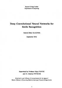
size 256. The initial learning rate is 0.001 and is reduced by a factor of 10 once after 10K iterations. For evaluation, we use 10-view testing [18]. We extract five 26 × 26 patches (the 4 corner patches and the center patch) as well as their horizontal reflections and average their predictions. The CIFAR100-NIN net obtains 35.27% testing error. Our HD-CNN achieves a testing error of 32.62%, which improves the building block net by 2.65%. Category hierarchy. During the construction of the category hierarchy, the number of coarse categories can be adjusted by the clustering algorithm. We can also make the coarse categories either disjoint or overlapping by varying the hyperparameter γ. Thus, we investigate their impacts on the classification error. We experiment with 5, 9, 14, and 19 coarse categories and vary the value of γ. The best results are obtained with 9 overlapping coarse categories and γ = 5, as shown in Fig 2 left. A histogram of fine category occurrences in 9 overlapping coarse categories is shown in Fig 2 right. The optimal value of coarse category number and hyperparameter γ are dataset dependent, mainly affected by the inherent hierarchy within the categories.

7.1. Overview We evaluate HD-CNN on CIFAR100 [17] and ImageNet [4]. HD-CNN is implemented on the widely deployed Caffe [15] software. The network is trained by back propagation [18]. We run all the testing experiments on a single NVIDIA Tesla K40c card.

Disjoint coarse categories Overlapping coarse categories, γ = 5 Overlapping coarse categories, γ = 10

35.5

25 20

35 34.5

15

34

10

33.5

7.2. CIFAR100 The CIFAR100 dataset consists of 100 classes of natural images. There are 50K training images and 10K testing images. We follow [11] to preprocess the dataset (e.g., global contrast normalization and ZCA whitening). Randomly cropped and flipped image patches of size 26 × 26 are used for training. We adopt a NIN network 1 with three stacked layers [21]. We denote it as CIFAR100-NIN, which will be the HD-CNN building block. Fine category components share preceding layers from conv1 to pool1, which accounts for 6% of the total parameters and 29% of the total floating point operations. The remaining layers are used as independent layers. For building the category hierarchy, we randomly choose 10K images from the training set as the held-out set. Fine categories within the same coarse categories are visually more similar. We pretrain the rear layers of fine category components. The initial learning rate is 0.01, and it is decreased by a factor of 10 every 6K iterations. Fine-tuning is performed for 20K iterations with large mini-batches of 1 https://github.com/mavenlin/cuda-convnet/blob/ master/NIN/cifar-100_def

5

33 5

10 15 20 number of coarse categories

0 0 1 2 3 4 5 6 7 8 fine category occurrences

Figure 2: Left: HD-CNN 10-view testing error against the number of coarse categories on CIFAR100. We pick 9 coarse categories and γ = 5. Right: Histogram of fine category occurrences in 9 overlapping coarse categories. Shared layers. The use of shared layers makes both the computational complexity and memory footprint of HDCNN sublinear in the number of fine category classifiers when compared to the building block net. Our HD-CNN with 9 fine category classifiers based on CIFAR100-NIN consumes less than three times as much memory as the building block net without parameter compression. We also want to investigate the impact of the use of shared layers on the classification error, memory footprint, and the net execution time (Table 2). We build another HDCNN, where coarse category component and all fine category components use independent preceding layers initialized from a pretrained building block net. Under singleview testing where only a central cropping is used, we ob-

Table 1: 10-view testing errors on CIFAR100 dataset. Notation CCC=coarse category consistency. Method Error Model averaging (2 CIFAR100-NIN nets) DSN [19] CIFAR100-NIN-double dasNet [30]

35.13 34.68 34.26 33.78

Base: CIFAR100-NIN HD-CNN, no fine-tuning HD-CNN, fine-tuning HD-CNN+CE+PC, fine-tuning

35.27 33.33 32.62 32.79

serve a minor error increase from 34.36% to 34.50%. But using shared layers dramatically reduces the memory footprint from 1356 MB to 459 MB and testing time from 2.43 seconds to 0.28 seconds. Conditional execution. By varying the hyperparameter β, we can effectively affect the number of fine category components that will be executed. There is a trade-off between execution time and classification error. A larger value of β leads to higher accuracy at the cost of executing more components for fine categorization. By enabling conditional executions with hyperparameter β = 6, we obtain a substantial 2.8x speedup with merely a minor increase in error from 34.36% to 34.57% (Table 2). The testing time of HD-CNN is about 2.5x as much as that of the building block net. Parameter compression. As fine category CNNs have independent layers from conv2 to cccp6, we compress them and reduce the memory footprint from 447MB to 286MB with a minor increase in error from 34.57% to 34.73%. Comparison with a strong baseline. As our HD-CNN memory footprint is about two times as much as the building block model (Table 2), it is necessary to compare a stronger baseline of similar complexity with HD-CNN. We adapt CIFAR100-NIN and double the number of filters in all convolutional layers, which accordingly increases the memory footprint by three times. We denote it as CIFAR100-NINdouble and obtain an error of 34.26%, which is 1.01% lower than that of the building block net but is 1.64% higher than that of HD-CNN. Comparison with model averaging. HD-CNN is fundamentally different from model averaging [18]. In model averaging, all models are capable of classifying the full set of the categories, and each one is trained independently. The main sources of their prediction differences are different initializations. In HD-CNN, each fine category classifier only excels at classifying a partial set of categories. To compare HD-CNN with model averaging, we independently train two CIFAR100-NIN networks and take their averaged prediction as the final prediction. We obtain an error

of 35.13%, which is about 2.51% higher than that of HDCNN (Table 1). Note that HD-CNN is orthogonal to the model averaging and an ensemble of HD-CNN networks can further improve the performance. Coarse category consistency. To verify the effectiveness of coarse category consistency term in our loss function (5), we fine-tune a HD-CNN using the traditional multinomial logistic loss function. The testing error is 33.21%, which is 0.59% higher than that of a HD-CNN fine-tuned with coarse category consistency (Table 1). Comparison with state-of-the-art. Our HD-CNN improves on the current two best methods [19], and [30], by 2.06% and 1.16%, respectively, and sets new state-ofthe-art results on CIFAR100 (Table 1).

7.3. ImageNet 1000 The ILSVRC-2012 ImageNet dataset consists of about 1.2 million training images, 50, 000 validation images. To demonstrate the generality of HD-CNN, we experiment with two different building block nets. In both cases, HDCNNs achieve significantly lower testing errors than the building block nets. 7.3.1

Network-In-Network Building Block Net

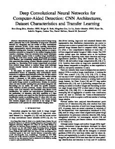
We choose a public 4-layer NIN net2 as our first building block, as it has a greatly reduced number of parameters compared to AlexNet [18] but similar error rates. It is denoted as ImageNet-NIN. In HD-CNN, various components share preceding layers from conv1 to pool3, which account for 26% of the total parameters and 82% of the total floating point operations. We follow the training and testing protocols as in [18]. Original images are resized to 256 × 256. Randomly cropped and horizontally reflected 224 × 224 patches are used for training. At test time, the net makes a 10-view averaged prediction. We train ImageNet-NIN for 45 epochs. The top-1 and top-5 errors are 39.76% and 17.71%, respectively. To build the category hierarchy, we take 100K training images as the held-out set and find 89 overlapping coarse categories. Each fine category CNN is fine-tuned for 40K iterations while the initial learning rate 0.01 is decreased by a factor of 10 every 15K iterations. Fine-tuning the complete HD-CNN is not performed, as the required minibatch size is significantly higher than that for the building block net. Nevertheless, we still achieve top-1 and top-5 errors of 36.66% and 15.80% and improve the building block net by 3.1% and 1.91%, respectively (Table 3). The classwise top-5 error improvement over the building block net is shown in Fig 4 left. 2 https://gist.github.com/mavenlin/ d802a5849de39225bcc6

hermit crab

hand blower

digital clock

ice lolly

(a)

alligator lizard scorpion crayfish fiddler crab tarantula 0 plunger barbell punching bag dumbbell power drill 0 odometer laptop projector cab notebook 0 bubble sunglasses sunglass cinema whistle 0

1

1

1

1

CC 6 CC 11 CC 10 CC 7 CC 82 0 CC 49 CC 74 CC 40 CC 81 CC 50 0 CC 65 CC 72 CC 75 CC 53 CC 63 0 CC 62 CC 75 CC 78 CC 50 CC 59 0

(b)

1

1

1

1

hermit crab alligator lizard fiddler crab banded gecko cricket 0 punching bag hand blower hair spray plunger barbell 0 iPod odometer pool table notebook digital clock 0 maypole umbrella ice lolly garbage truck scoreboard 0

(c)

1

1

1

1

(d)

tarantula ringneck snake hermit crab banded gecko alligator lizard 0 hand blower punching bag hair spray maraca barbell 0 monitor odometer laptop digital clock iPod 0 ice lolly sunglass sunglasses plunger maraca 0

hermit crab thunder snake scorpion gar banded gecko 1 0 punching bag dumbbell hair spray hand blower maraca 1 0 laptop digital clock Polaroid camera ski mask traffic light 1 0 ice lolly bow tie whistle maypole cinema 1 0

(e)

1

1

1

1

(f)

hermit crab tarantula fiddler crab alligator lizard ringneck snake 0 hand blower punching bag hair spray plunger dumbbell 0 digital clock laptop odometer iPod projector 0 ice lolly sunglass sunglasses umbrella maypole 0

1

1

1

1

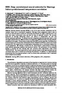
(g)

Figure 3: Case studies on ImageNet dataset. Each row represents a testing case. Column (a): test image with ground truth label. Column (b): top 5 guesses from the building block net ImageNet-NIN. Column (c): top 5 Coarse Category (CC) probabilities. Column (d)-(f): top 5 guesses made by the top 3 fine category CNN components. Column (g): final top 5 guesses made by the HD-CNN. See text for details. Table 2: Comparison of testing errors, memory footprint (MB) and testing time (seconds) between building block nets and HD-CNNs on CIFAR100 and ImageNet datasets. Statistics are collected under single-view testing. Three building block nets, CIFAR100-NIN, ImageNet-NIN, and ImageNet-VGG-16-layer, are used. The testing mini-batch size is 50. Notations: SL=Shared layers, CE=Conditional execution, PC=Parameter compression. Model

top-1, top-5

Memory Time

Base:CIFAR100-NIN HD-CNN w/o SL HD-CNN HD-CNN+CE HD-CNN+CE+PC

37.29 34.50 34.36 34.57 34.73

188 1356 459 447 286

0.04 2.43 0.28 0.10 0.10

Base:ImageNet-NIN HD-CNN HD-CNN+CE HD-CNN+CE+PC

41.52, 18.98 37.92, 16.62 38.16, 16.75 38.39, 16.89

535 3544 3508 1712

0.19 3.25 0.52 0.53

Base:ImageNet-VGG16-layer HD-CNN+CE+PC

32.30, 12.74

4134

1.04

31.34, 12.26

6863

5.28

Case studies. We want to investigate how HD-CNN corrects the mistakes made by the building block net. In Fig 3, we collect four testing cases. In the first case, the building block net fails to predict the label of the tiny hermit crab in the top 5 guesses. In HD-CNN, two coarse categories, #6 and #11, receive most of the coarse probability mass. The fine category component #6 specializes in classifying crab breeds and strongly suggests the ground truth label. By combining the predictions from the top fine category clas-

sifiers, the HD-CNN predicts hermit crab as the most probable label. In the second case, the ImageNet-NIN confuses the ground truth hand blower with other objects of close shapes and appearances, such as plunger and barbell. For HD-CNN, the coarse category component is also not confident about which coarse category the object belongs to and thus assigns even probability mass to the top coarse categories. For the top 3 fine category classifiers, #74 strongly predicts ground truth label while the other two ,#49 and #40, rank the ground truth label at the 2nd and 4th place, respectively. Overall, the HD-CNN ranks the ground truth label at the 1st place. This demonstrates HD-CNN needs to rely on multiple fine category classifiers to make correct predictions for difficult cases. Overlapping coarse categories.To investigate the impact of overlapping coarse categories on the classification, we train another HD-CNN with 89 fine category classifiers using disjoint coarse categories. It achieves top-1 and top-5 errors of 38.44% and 17.03%, respectively, which is higher than those of the HD-CNN using an overlapping coarse category hierarchy by 1.78% and 1.23% (Table 3). Conditional executions. By varying the hyperparameter β, we can control the number of fine category components that will be executed. There is a trade-off between execution time and classification error, as shown in Fig 4 right. A larger value of β leads to lower error at the cost of more executed fine category components. By enabling conditional executions with hyperparameter β = 8, we obtain a substantial 6.3x speedup with merely a minor increase of single-view testing top-5 error from 16.62% to 16.75% (Table 2). With such speedup, the HD-CNN testing time is less than 3 times as much as that of the building block net. Parameter compression. We compress independent layers conv4 and cccp7, as they account for 60% of the parameters in ImageNet-NIN. Their parameter matrices are of size

Table 3: Comparisons of 10-view testing errors between ImageNet-NIN and HD-CNN. Notation CC=Coarse category. Method

top-1, top-5

Base:ImageNet-NIN Model averaging (3 base nets) HD-CNN, disjoint CC HD-CNN HD-CNN+CE+PC

39.76, 17.71 38.54, 17.11 38.44, 17.03 36.66, 15.80 36.88, 15.92

Mean # of executed components

error improvement

0.2 0.1 0.0 −0.1 −0.2

−0.3 0

200

400

class

600

800

1000

12

0.18

10

0.175

8

0.17

6

0.165

4

0.16

2

0.155

0 -5

-4

-3

-2

-1

0

log β

1

2

3

4

2

Comparison with model averaging. As the HD-CNN memory footprint is about three times as much as the building block net, we independently train three ImageNet-NIN nets and average their predictions. We obtain a top-5 error 17.11%, which is 0.6% lower than the building block but is 1.31% higher than that of HD-CNN (Table 3). VGG-16-layer Building Block Net

The second building block net we use is a 16-layer CNN from [26]. We denote it as ImageNet-VGG-16-layer3 . The layers from conv1 1 to pool4 are shared, and they account for 5.6% of the total parameters and 90% of the total floating number operations. The remaining layers are used as independent layers in coarse and fine category classifiers. We follow the training and testing protocols as in [26]. For training, we first sample a size S from the range [256, 512] and resize the image so that the length of the short edge is S. Then a randomly cropped and flipped patch of size 224 × 224 is used for training. For testing, dense evaluation is performed on three scales {256, 384, 512}, and the averaged prediction is used as the final prediction. Please 3 https://github.com/BVLC/caffe/wiki/Model-Zoo

Table 4: Errors on ImageNet validation set. Method

top-1, top-5

GoogLeNet,multi-crop [31] VGG-19-layer, dense [26] VGG-16-layer+VGG-19-layer,dense

N/A,7.9 24.8,7.5 24.0,7.1

Base:ImageNet-VGG-16-layer,dense HD-CNN+PC,dense HD-CNN+PC+CE,dense

24.79,7.50 23.69,6.76 23.88,6.87

0.15

Figure 4: Left: Class-wise HD-CNN top-5 error improvement over the building block net. Right: Mean number of executed fine category classifiers and top-5 error against hyperparameter β on the ImageNet validation dataset.

7.3.2

Top 5 error

1024 × 3456 and 1024 × 1024 and we use compression hyperparameters (s, k) = (3, 128) and (s, k) = (2, 256). The compression factors are 4.8 and 2.7. The compression decreases the memory footprint from 3508MB to 1712MB and merely increases the top-5 error from 16.75% to 16.89% under single-view testing (Table 2).

refer to [26] for more training and testing details. On the ImageNet validation set, ImageNet-VGG-16-layer achieves top-1 and top-5 errors of 24.79% and 7.50% respectively. We build a category hierarchy with 84 overlapping coarse categories. We implement multi-GPU training on Caffe by exploiting data parallelism [26] and train the fine category classifiers on two NVIDIA Tesla K40c cards. The initial learning rate is 0.001, and it is decreased by a factor of 10 every 4K iterations. HD-CNN fine-tuning is not performed. Due to the large memory footprint of the building block net (Table 2), the HD-CNN with 84 fine category classifiers cannot fit into the memory directly. Therefore, we compress the parameters in layers fc6 and fc7 as they account for over 85% of the parameters. Parameter matrices in fc6 and fc7, are of size 4096 × 25088 and 4096 × 4096. Their compression hyperparameters are (s, k) = (14, 64) and (s, k) = (4, 256). The compression factors are 29.9 and 8, respectively. The HD-CNN obtains top-1 and top-5 errors of 23.69% and 6.76% on the ImageNet validation set and improves over ImageNet-VGG-16-layer by 1.1% and 0.74%, respectively.

Comparison with state-of-the-art. Currently, the two best nets on the ImageNet dataset are GoogLeNet [31] (Table 4) and VGG 19-layer network [26]. Using multi-scale multicrop testing, a single GoogLeNet net achieves a top-5 error of 7.9%. With multi-scale dense evaluation, a single VGG 19-layer net obtains top-1 and top-5 errors of 24.8% and 7.5% and improves the top-5 error of GoogLeNet by 0.4%. Our HD-CNN decreases the top-1 and top-5 errors of VGG 19-layer net by 1.11% and 0.74%, respectively. Furthermore, HD-CNN slightly outperforms the results of averaging the predictions from VGG-16-layer and VGG-19-layer nets.

8. Conclusions and Future Work We demonstrated that HD-CNN is a flexible deep CNN architecture to improve over existing deep CNN models. We showed this empirically on both CIFAR-100 and ImageNet datasets using three different building block nets. As part of our future work, we plan to extend HD-CNN architectures to those with more than 2 hierarchical levels and also verify our empirical results in a theoretical framework.

References [1] H. Bannour and C. Hudelot. Hierarchical image annotation using semantic hierarchies. In Proceedings of the 21st ACM International Conference on Information and Knowledge Management, 2012. [2] S. Bengio, J. Weston, and D. Grangier. Label embedding trees for large multi-class tasks. In NIPS, 2010. [3] J. Deng, N. Ding, Y. Jia, A. Frome, K. Murphy, S. Bengio, Y. Li, H. Neven, and H. Adam. Large-scale object classification using label relation graphs. In ECCV. 2014. [4] J. Deng, W. Dong, R. Socher, L. Li, K. Li, and F. Li. Imagenet: A large-scale hierarchical image database. In CVPR, 2009. [5] J. Deng, J. Krause, A. C. Berg, and L. Fei-Fei. Hedging your bets: Optimizing accuracy-specificity trade-offs in large scale visual recognition. In CVPR, 2012. [6] J. Deng, S. Satheesh, A. C. Berg, and F. Li. Fast and balanced: Efficient label tree learning for large scale object recognition. In Advances in Neural Information Processing Systems, 2011. [7] C. Farabet, C. Couprie, L. Najman, and Y. LeCun. Learning hierarchical features for scene labeling. IEEE Transactions on Pattern Analysis and Machine Intelligence, 2013. [8] R. Fergus, H. Bernal, Y. Weiss, and A. Torralba. Semantic label sharing for learning with many categories. In ECCV. 2010. [9] T. Gao and D. Koller. Discriminative learning of relaxed hierarchy for large-scale visual recognition. In ICCV, 2011. [10] R. Girshick, J. Donahue, T. Darrell, and J. Malik. Rich feature hierarchies for accurate object detection and semantic segmentation. In CVPR, 2014. [11] I. Goodfellow, D. Warde-Farley, M. Mirza, A. Courville, and Y. Bengio. Maxout networks. In ICML, 2013. [12] G. Griffin and P. Perona. Learning and using taxonomies for fast visual categorization. In CVPR, 2008. [13] K. He, X. Zhang, S. Ren, and J. Sun. Spatial pyramid pooling in deep convolutional networks for visual recognition. In ECCV. 2014. [14] H. Jegou, M. Douze, and C. Schmid. Product quantization for nearest neighbor search. IEEE Transactions on Pattern Analysis and Machine Intelligence, 2011. [15] Y. Jia. Caffe: An open source convolutional architecture for fast feature embedding, 2013. [16] Y. Jia, J. T. Abbott, J. Austerweil, T. Griffiths, and T. Darrell. Visual concept learning: Combining machine vision and bayesian generalization on concept hierarchies. In NIPS, 2013. [17] A. Krizhevsky and G. Hinton. Learning multiple layers of features from tiny images. Computer Science Department, University of Toronto, Tech. Rep, 2009. [18] A. Krizhevsky, I. Sutskever, and G. Hinton. Imagenet classification with deep convolutional neural networks. In NIPS, 2012. [19] C.-Y. Lee, S. Xie, P. Gallagher, Z. Zhang, and Z. Tu. Deeplysupervised nets. arXiv preprint arXiv:1409.5185, 2014.

[20] L.-J. Li, C. Wang, Y. Lim, D. M. Blei, and L. Fei-Fei. Building and using a semantivisual image hierarchy. In CVPR, 2010. [21] M. Lin, Q. Chen, and S. Yan. Network in network. CoRR, 2013. [22] B. Liu, F. Sadeghi, M. Tappen, O. Shamir, and C. Liu. Probabilistic label trees for efficient large scale image classification. In CVPR, 2013. [23] M. Marszalek and C. Schmid. Semantic hierarchies for visual object recognition. In CVPR, 2007. [24] M. Marszałek and C. Schmid. Constructing category hierarchies for visual recognition. In ECCV. 2008. [25] R. Salakhutdinov, A. Torralba, and J. Tenenbaum. Learning to share visual appearance for multiclass object detection. In CVPR, 2011. [26] K. Simonyan and A. Zisserman. Very deep convolutional networks for large-scale image recognition. CoRR, abs/1409.1556, 2014. [27] J. Sivic, B. C. Russell, A. Zisserman, W. T. Freeman, and A. A. Efros. Unsupervised discovery of visual object class hierarchies. In CVPR, 2008. [28] J. T. Springenberg and M. Riedmiller. Improving deep neural networks with probabilistic maxout units. arXiv preprint arXiv:1312.6116, 2013. [29] N. Srivastava and R. Salakhutdinov. Discriminative transfer learning with tree-based priors. In NIPS, 2013. [30] M. F. Stollenga, J. Masci, F. Gomez, and J. Schmidhuber. Deep networks with internal selective attention through feedback connections. In NIPS, 2014. [31] C. Szegedy, W. Liu, Y. Jia, P. Sermanet, S. Reed, D. Anguelov, D. Erhan, V. Vanhoucke, and A. Rabinovich. Going deeper with convolutions. arXiv preprint arXiv:1409.4842, 2014. [32] A.-M. Tousch, S. Herbin, and J.-Y. Audibert. Semantic hierarchies for image annotation: A survey. Pattern Recognition, 2012. [33] N. Verma, D. Mahajan, S. Sellamanickam, and V. Nair. Learning hierarchical similarity metrics. In CVPR, 2012. [34] T. Xiao, J. Zhang, K. Yang, Y. Peng, and Z. Zhang. Errordriven incremental learning in deep convolutional neural network for large-scale image classification. In Proceedings of the ACM International Conference on Multimedia, 2014. [35] M. Zeiler and R. Fergus. Visualizing and understanding convolutional networks. In ECCV. 2014. [36] M. D. Zeiler and R. Fergus. Stochastic pooling for regularization of deep convolutional neural networks. In ICLR, 2013. [37] B. Zhao, F. Li, and E. P. Xing. Large-scale category structure aware image categorization. In NIPS, 2011. [38] A. Zweig and D. Weinshall. Exploiting object hierarchy: Combining models from different category levels. In ICCV, 2007.