Tree-CNN: A Hierarchical Deep Convolutional Neural Network for

Tree-CNN: A Hierarchical Deep Convolutional Neural Network for Incremental Learning

1 Department

Deboleena Roy1,2 , Priyadarshini Panda1 and Kaushik Roy1 of Electrical and Computer Engineering, Purdue University, West Lafayette, IN 47906 2 [email protected]

Abstract In recent years, Convolutional Neural Networks (CNNs) have shown remarkable performance in many computer vision tasks such as object recognition and detection. However, complex training issues, such as “catastrophic forgetting” and hyper-parameter tuning, make incremental learning in CNNs a difficult challenge. In this paper, we propose a hierarchical deep neural network, with CNNs at multiple levels, and a corresponding training method for incremental learning. The network grows in a tree-like manner to accommodate the new classes of data without losing the ability to identify the previously trained classes. The proposed network was tested on CIFAR-100 and reported 60.46% accuracy and 20% reduction in training effort as compared to retraining final layers of a deep network. The network organizes the incoming classes of data into feature-driven super-classes and improves upon existing hierarchical CNN models by adding the capability of self-growth.

1

Introduction

In recent years Deep Convolutional Neural Networks (DCNNs) have emerged as the leading architecture for large scale image classification [19]. In 2012, AlexNet [13] won the ImageNet Large Scale Visual Recognition Challenge (ISLVRC) by implementing a Deep-CNN and catapulted DCNNs into the spotlight. Since then, they have dominated ISLVRC and have performed extremely well on popular image datasets such as MNIST [14, 30], CIFAR-10/100 [12], and ImageNet [21]. Today, with increased access to large amount of labeled data (eg. ImageNet contains 1.2 million images with 1000 categories), supervised learning has become the leading paradigm in training DCNNs for image recognition. Traditionally, a DCNN is trained on a dataset containing large number of labeled images. The network learns to extract relevant features and classify these images. This trained model is then used on real world unlabeled images to classify them. In such training, all the training data is presented to the network during the same training process. However, in real world, we hardly have all the information at once. Instead, data is gathered incrementally over time. We need systems that can learn new tasks as new information is available. In this work, we try to address the challenge of incremental learning in the domain of image recognition using deep networks. A DCNN embeds feature extraction and classification in one coherent architecture within the same model. Modifying one part of the parameter space immediately affects the model globally. Another problem of incrementally training a DCNN is the issue of “catastrophic forgetting”[6]. When new data is fed into a DCNN, it results in the destruction of existing features learned from earlier data. This mandates using previous data when retraining on new data. To avoid catastrophic forgetting, and to leverage the features learned in previous task, this work proposes a network made of CNNs that grows hierarchically as new classes are introduced. The network adds the new classes like new leaves to the hierarchical structure. The branching is based on the similarity of features between new and old classes. The initial nodes of the Tree-CNN assign the Preprint. Work in progress.

input into coarse super-classes, and as we approach the leaves of the network, finer classification is done. Such a model allows us to leverage the convolution layers learned previously to be used in the new bigger network. The rest of the paper is organized as follows. The related work on incremental learning in deep neural networks is discussed in Section 2. In Section 3 we present our proposed network architecture and incremental learning method. In Section 4, the two experiments using CIFAR-10 and CIFAR-100 datasets are described. It is followed by a detailed analysis of the performance of the network and its comparison with basic transfer learning and fine tuning in Section 5. Finally, Section 6 discusses the merits and limitations of our network, and our findings and suggests opportunities for future work.

2

Related Work

The modern world of digitized data produces new information every second [10], thus fueling the need for systems that can learn as new data arrives. Traditional deep neural networks are static in that respect, and several new approaches to incremental learning are currently being explored. “One-shot learning” [4] is a Bayesian transfer learning technique, that uses very few training samples to learn new classes. Fast R-CNN [5], a popular framework for object detection, also suffers from “catastrophic forgetting”. One way to mitigate this issue is to use a frozen copy of the original network compute and balance the loss when new classes are introduced in the network[24]. "Learning without Forgetting" [15] is another method that uses only new task data to train the network while preserving the original capabilities. However, here the original network is trained on an extensive dataset, such as ImageNet [21], and the new task data is a much smaller dataset. ‘Expert Gate’ [1] adds networks (or experts) trained on new tasks sequentially to the system and uses a set of gating autoencoders to select the right network (‘expert’) for the given input. Progressive Neural Networks [22] learn to solve complex sequences of task by leveraging prior knowledge with lateral connections. Another recent work on incremental learning in neural networks is iCaRL [20], where they built an incremental classifier that can potentially learn incrementally over an indefinitely long time period. Transfer learning plays a significant role in incremental learning. It allows us to leverage past knowledge. It has been observed that initial layers of a CNN learn very generic features[33] [23]. Common features, that are shared between images, have been exploited to build hierarchical classifiers. These features can be grouped semantically, such as in [18], or be feature-driven, such as “FALCON” [17]. Similar to the progression of complexity of convolutional layers in a DCNN, the upper nodes of a hierarchical CNN classify the images into coarse super-classes using basic features, like grouping green-colored objects together, or humans faces together. Then deeper nodes perform finer discrimination, such as “boy” v/s “girl” , “apples” v/s “oranges”, etc. Such hierarchical CNN models have been shown to perform at par or even better than standard DCNNs [32]. “Discriminative Transfer learning” [28] is one of the earliest works where classes are categorized hierarchically to improve network performance. Deep Neural Decision Forests [11] unified decision trees and deep CNN’s to build a hierarchical classifier. “HD-CNN” [32], is a hierarchical CNN model that is built by exploiting the common feature sharing aspect of images. However, in these works, the dataset is fixed from the beginning, and prior knowledge of all the classes and their properties is used to build a hierarchical model. In this work, the Tree-CNN starts out as a single root node and generates new hierarchies to accommodate the new classes. Images belonging to the older dataset are required during retraining, but by localizing the change to a small section of the whole network, our method tries to reduce the training effort and complexity. In [31], a similar approach is applied, where the new classes are added to the old classes, and divided into two super-classes, by using an error-based model. The initial network is cloned to form two new networks which are fine tuned over the two new super-classes. While their motivation was a "divide-and-conquer" approach for large datasets, this work tries to incrementally grow with new data. And, we sequentially add new data over multiple learning stages. In the next section, we lay out in detail our design principle, network topology and the algorithm used to grow the network. 2

IMAGE

Root Node classifies input image into one of the “superclasses”

Branch Node Fine classifier

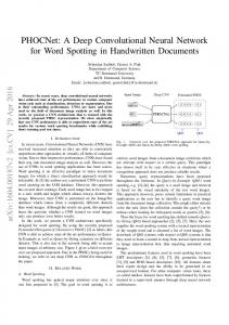
Figure 1: A generic model of Tree-CNN: The root node predicts super-classes whereas lower nodes predict finer classes

3

Incremental Learning Model

The Tree-CNN is made of nodes connected as a directed acyclic graph. Each node acts a classifier that outputs a label for the input image. As per the label, the image is then passed on to the next node which further classifies the image, until we reach a leaf node, the last step of classification. The root node is the highest node of the tree. The first classification happens at this node. Next in hierarchy is the branch node. It has a parent and two or more children. It performs classification for at minimum 2 classes/super-classes. The leaf node is the last level of the tree. Each leaf node is uniquely associated to a class. No two leaf nodes have the same class. Fig. 1 shows the root node and branch nodes for a two-stage classification network. Each output of the second level branch node is a leaf node. The network starts out as a single node that can classify N classes. This is the first task the network learns. The CNN is trained using gradient descent and back-propagation on training images belonging to those N classes. A new task arrives which requires the system to classify M new classes. A small sample of images (∼ 10%) is selected from the training set of the new classes. At the root node these images are fed to the DCNN, one class at a time. We obtain a 3 dimensional matrix, O K×M×I , where, K is number of children of the root node, M is number of new classes, and I number of sample images per class. O(k, m, i) denotes the output of the k th output neuron for the i th image belonging K×M is the average of the outputs over to the mth class where k ∈ [1, K], m ∈ [1, M], and i ∈ [1, I]. O avg I images . Softmax is taken over O avg to obtain the likelihood matrix L K×M 1. Each column of L can be represented as a K × 1 vector, l m , where m ∈ [1, M] represents the M new classes. We arrange l m in an ordered set, S as given by 2. O avg (k, m) =

I Õ O(k, m, i)

I

i=1

and

L(k, m) =

eOav g (k,m) K Í eOav g (k,m)

(1)

k=1

S = [l m1, l m2, ...l mM ] ,

max(l m1 (k)) >= max(l m2 (k)) >= ... >= max(l mM (k)) k

k

k

(2)

The ordering is done so that new classes with high likelihood values are attended to first. A class with a high max(l m (k)) like 0.9 indicates that it has a strong affinity to a particular child node. So we first add that class. A class with a low max(l m (k)) such as 0.2 indicates it probably has almost equal likelihood of being classified to any of the nodes. Softmax likelihood is used instead of counting how many images get classified to one of the child nodes because it translates the image’s response to the child nodes into an exponential scale and captures how strongly a child node responds to an image of a particular class, rather than if it is the highest of all nodes. Once we have S, we go through it in an ordered manner and take one of the 3 actions: i. Add the new class to an existing child node: If the value of max(l m ) is greater than a threshold (a design specification), it indicates a strong resemblance/association with a particular child node. The new class is added to child node k such that l m (k) = max (l m (k 0)), k 0 ∈ 0 k

[1, K] 3

ii. Combine one or more child nodes and the new class to form a new child node: If there are more than 1 child nodes that the new class has a strong likelihood for, we can combine them to form a new child node. Say, the top two likelihood values were 0.48,and 0.45, and at least one of them is a leaf node, we can combine the two and the new class to form a new child node which will be a branch node. We can set an upper limit to the number of child nodes that could be combined iii. Add the new class as a new child node: If the new class doesn’t have a single likelihood value greater than a threshold (l m (i) < threshold ∀i ∈ [1, K]), or certain network restrictions are applied to prevent addition of classes to child nodes, the network expands horizontally by adding the new class as a new child node. This node will be a leaf node. Once this is complete for the M classes at the root node, we move to the next level of the tree. The same process is applied on the child nodes that now have new classes to be added to them. As we move to the next level, the sample images belonging to the only those new classes that are assigned to a particular child node are shown to it. Overall, for one level, sample images of all M classes are passed through different child nodes. For example, say, two new classes were added to a child node. If child node is a leaf node, it is changed into a branch node that now has 3 leaf nodes as children. If the child node is a branch node, then we repeat the process of calculating likelihood matrix and determining how these two new classes will get added to its output. The decision on how to grow the tree is semi-supervised: the algorithm itself decides how to grow the tree, given the constraints by the user. We can limit parameters such as maximum children for a node, maximum depth for the tree, etc. as per our system requirements. Once the new classes are allotted locations in the tree, supervised gradient descent based training is performed on the modified/new nodes. This saves us from modifying the whole network, and only affected portions of the network require retraining/fine-tuning.

4

Experiments

We conducted two experiments using the datasets CIFAR-10 and CIFAR-100[12], and used MatConvNet [29], an open-source toolbox for implementation of Convolutional Neural Networks in MATLAB [16]. During training, data augmentation was done by flipping the training images horizontally at random with a probability of 0.5 [7]. All images were whitened and contrast normalized [7]. The activation used in all the networks is rectified linear activation ReLU, σ(x) = max(x, 0). The networks are trained using stochastic gradient descent with fixed momentum of 0.9. Dropout [27] is used between the final fully connected layers, and between pooling layers to regularize the network. We also employed batch-normalization (BNORM) [9] at the output of every convolutional layer. Additionally, a weight decay λ = 0.001 was set to regularize each model. The weight decay helps against overfitting of our model. The final layer performs softmax operation on the output of the nodes to generate class probabilities. All CNNs are trained for 300 epochs. The learning rate is kept at 0.1 for first 200 epochs, then reduced by 10 times every 50 epochs. There is an absence of standardized benchmark protocol for incremental learning. A benchmark protocol similar to one used in iCaRL[20] is used here. The classes of the dataset are arranged in a fixed random order. After each incremental learning stage, the network would be evaluated on the classes it has already been trained on and the accuracy would be reported. To compare against the Tree-CNN, we took another network (Network “B”) with a complexity level similar to two stage complexity of this Tree-CNN. It has 4 convolutional blocks, each block having 2 sets of 3 × 3 convolutional kernels. The network is inspired from the architecture of VGG-net [25]. Detailed model is given in Table 3. This is also trained in incremental stages using fine-tuning. The new classes are added as new output nodes of the final layer and 5 different fine tuning strategies have been used. Each method retrains/fine-tunes certain layers of the network. As listed below, we set 5 different depths of back-propagation when retraining with the incremental + old dataset. 1. 2. 3. 4.

Case I: FC Case II: FC + CONV1 Case III: FC + CONV1 + CONV2 Case IV: FC + CONV1 + CONV2 + CONV3 4

5. Case V: FC + CONV1 + CONV2 + CONV3 + CONV4 (equivalent to training a new network with all the classes) We compare our Tree-CNN Íagainst retraining network ‘B’ on two metrics: Testing Accuracy, and Training Effort , which is (total number of weights × total number of training samples) nets

Training Effort tries to capture the number of weight updates that happen per training epoch. As batch size and number of training epochs is kept the same, the product of number of weights and the number of training samples used gives us a good measure of the effort used in training a network. This metric allows us to compare the computational effort without making it specific to a particular hardware on which the computation is performed. For Tree-CNN the training effort of each of the nodes (‘nets’) is summed together. For network “B”, there is only one net in each case. 4.1

Adding Multiple New Classes

Dataset CIFAR-10 dataset [12], having 10 mutually exclusive classes, was used for this experiment. The network is first trained on 6 classes, and then learns the remaining 4 classes as an incremental learning stage. Network For ease of reference, we label this network as Tree-CNN A. The root node is a DCNN with two output nodes. It will classify the input image as either “Animals” or “Vehicles”. Each child node has a DCNN that does finer classification. The detailed description of the layers in each of these sub-networks can be found in the supplementary section. Fig. 2 and Fig. 3 a) depict the initial model of Tree-CNN A. This experiment is used to demonstrate how the network grows in a simplistic manner. It demonstrates at given intermediate Tree-CNN state, how it would respond to new classification data. a)

b)

ROOT

ROOT

“Vehicle”

FC

FC

CONV 3

CONV 2

LEAF NODES

ANIMAL

VEHICLE

ANIMAL

VEHICLE

SHIP

CAT

SHIP

CAT

DOG

TRUCK

DOG

TRUCK

HORSE

AUTOMOBILE

HORSE

AUTOMOBILE

DEER

AEROPLANE

NEW CLASSES

FC

CONV 3

CONV 2

“Animal”

CONV 1

CONV 2

CONV 1

IMAGE 32x32x3 RGB

CONV 1

BRANCH NODES

“Root”

BIRD FROG

Figure 2: Detailed network of Tree-CNN A (before incremental learning)

Figure 3: Graphical representation of Tree-CNN A a) before incremental learning, b) after incremental learning

Initial Training 6 classes of CIFAR-10 are grouped into “Vehicles” and “Animals” as shown in Fig 3. The root node achieves a testing accuracy of 98.73%, while the branch nodes, “Animals” and “Vehicles”, achieve 86% and 94.43% testing accuracy respectively. Overall, this network achieves a testing accuracy of 89.10%. Network “B” is trained on the 6 image classes and achieves a testing accuracy of 92.40%. Incremental Learning The remaining four classes are now introduced as the new incremental task. 50 images (10% of the training set) per class are selected at random , and shown to the root node. We obtain the L matrix, which is a 2 × 4 matrix with each element l i j ∈ (0, 1). The 1st row of the matrix indicates the softmax likelihood of each of the 4 classes as being classified as “Vehicles”, while the second row presents the same information for “Animals”. In this experiment, the network takes one action: Add the new class to an existing child node and threshold is set at 0.5. The before and after structure of the Tree-CNN A is shown in Fig. 3 . Next the root node is retrained with 50, 000 training images from all the 10 classes(old and new) to classify them in to the two coarse categories. Then the two branch nodes are trained. 5

4.2

Sequentially Adding Multiple Classes

Dataset For this experiment, CIFAR-100 [12] is used. It has 100 classes, 500 training and 100 testing images per class. The 100 classes are divided into 10 groups of 10 classes each and organized in a fixed random order, details of which are provided in the supplementary section. The network is trained incrementally on these groups of classes. The first experiment was a proof of concept where we showed how a small tree-like structure would grow. Here there is no fixed hierarchical grouping of classes, unlike earlier. The aim is to show this method works irrespective of the initial grouping. The Network Initially, the Tree-CNN has a root node and 10 leaf nodes. We label this network as Tree-CNN C. The root node has a DCNN network, with 10 output nodes. The layers of the CNN are described in detail in Table 1. In subsequent learning stages, the network would extend branches. The DCNN model used in branch nodes is given in Table 2. The branch node is at more risk of overfitting than the root node. The dataset size shrinks as we move deeper into the tree. Hence lower nodes require more regularization techniques. In this network, we added more dropout layers in the branch node CNN to compensate overfitting. Table 1: Root Node Tree-CNN C

Table 2: Branch Node TreeCNN C

Input 32x32x3 Conv 1 5x5x3x64 ReLU stride 1 + BNORM [2 2] Max Pooling stride 2 Conv 2 3x3x64x128 ReLU stride 1 + BNORM Dropout 0.5 3x3x128x128 ReLU stride 1 + BNORM [2 2] Max Pooling stride 2 Conv 3 3x3x128x256 ReLU stride 1 + BNORM Dropout 0.5 3x3x256x256 ReLU stride 1 + BNORM [2 2] Avg Pooling stride 2 FC Fully Connected 4x4x256x1024 ReLU Dropout 0.5 Fully Connected 1x1x1024x1024 ReLU Dropout 0.5 Fully Connected 1x1x1024xN (N = Number of Children)

Input 32x32x3 Conv 1 5x5x3x32 ReLU stride 1 + BNORM [2 2] Max Pooling stride 2 Dropout 0.25 Conv 2 5x5x32x64 ReLU stride 1 + BNORM [2 2] Max Pooling stride 2 Dropout 0.25 Conv 3 3x3x64x64 ReLU stride 1 + BNORM Dropout 0.5 3x3x256x256 ReLU stride 1 + BNORM [2 2] Avg Pooling stride 2 FC Fully Connected 4x4x64x512 ReLU Dropout 0.5 Fully Connected 1x1x512x128 ReLU Dropout 0.5 Fully Connected 1x1x128xN (N = Number of Children)

Table 3: Network B Input 32x32x3 Conv1 3x3x3x64 ReLU stride 1 + BNORM Dropout 0.5 3x3x64x64 ReLU stride 1 + BNORM [2 2] Max Pooling stride 2 Conv 2 3x3x64x128 ReLU stride 1 + BNORM Dropout 0.5 3x3x128x128 ReLU stride 1 + BNORM [2 2] Max Pool stride 2 Conv3 3x3x128x256 ReLU stride 1 + BNORM Dropout 0.5 3x3x256c256 ReLU stride 1 + BNORM [2 2] Max pooling stride 2 Conv4 3x3x256x512 ReLU stride 1 + BNORM Dropout 0.5 3x3x512x512 ReLU stride 1 + BNORM [2 2] Avg Pooling stride 2 FC Fully Connected 2x2x512x1024 ReLU Dropout 0.5 Fully Connected 1x1x1024x1024 ReLU Dropout 0.5 Fully Connected 1x1x1024xN (N=Number of Classes)

Initial Training For Tree-CNN C, the root node is trained to classify 10 classes and it records a testing accuracy of 84.90%. Network “B” achieves a testing accuracy of 85%. Thus the starting accuracy for the two networks is almost the same. Incremental Learning We divided the remaining 90 classes into 9 groups, each containing 10 classes. These classes were added to the network in 9 incremental learning stages. At each stage, first 50 images belonging to each class are shown to the root node and a likelihood matrix L is generated. The columns of the matrix are used to form an ordered set S, as described in equation 2. For this experiment, we applied the following constraints to the system: • Maximum depth of the tree is 2. • Maximum number of output/children for a branch node is 10 It was observed during developing the algorithm that new classes tend to have a higher softmax likelihood value for branch nodes with higher number of children. To prevent the network from being lop-sided, by having one very large branch, we limit the number of children to 10 per branch 6

node. Once the placement of the new classes is determined we train the root node and the modified branch nodes. The pseudo-code of how we grow the network is given by Algorithm 1. We sort the "likelihood" array, l in descending order and store the value and the index. The index holds the corresponding number of the child node. We use the top 3 values of the likelihood array to determine how the mt h new class would be added to the tree. The various threshold used for comparing the softmax values are required to be set externally depending on the network environment. Network B is also trained in 5 different manners on the 10 incremental batches of data. Algorithm 1 Grow Tree-CNN C 1: S is the Likelihood matrix 2: procedure G ROW T REE(S, Tree-CNN) 3: for m in (1, M) do 4: l = S(m) and set l( j) = 0 for full child nodes j 5: val, ind = sort(l, ‘descend’) 6: if val(1) > 0.55 then add class m to node ind(1), continue 7: end if 8: if val(1) − val(2) < 0.1 and val(2) − val(3) > 0.1 then 9: merge ind(1) and ind(2) 10: add new class m to the merged node, continue 11: else 12: create new child node, add class m to new node 13: end if 14: end for 15: end procedure

5

Results

Adding multiple new classes (CIFAR-10) In Table 4, we report the test accuracy and the training effort for the 5 cases of fine-tuning network “B” against our Tree-CNN C for CIFAR-10. Fig. 3b shows the graphical structure of Tree-CNN A after addition of new classes. Retraining only FC layer of network “B” requires the least training effort. However, it gives us the lowest accuracy, 78.37% amongst all. And as more classes are introduced, this method causes much loss in accuracy, as shown with CIFAR-100 in Fig. 5. Our proposed model, Tree-CNN A has the second lowest normalized training effort, ∼ 40% less than ‘B:V’, and ∼ 30% less than ‘B:II’. At the same time, Tree-CNN A (86.25%) had comparable accuracy to ‘B:II’ (85.02%) and ‘B:III’ (88.15%), while just being less than the ideal case ‘B:V’ by a margin of 3.76%. Table 4: Training Effort and Test Accuracy comparison for CIFAR-10 dataset B:I B:II B:III Testing Accuracy 78.37 85.02 88.15 Normlaized Training Effort 0.40 0.85 0.96

Tree-CNN A against Network B for B:IV 90.00 0.99

B:V 90.51 1

Tree-CNN A 86.24 0.60

Sequentially adding new classes (CIFAR-100) We compare Tree-CNN C against the 5 different fine-tuning cases of Network B. Fig. 4 shows the training effort. We normalized the training effort by dividing all the values with the highest training effort. i.e. B:V. B:I has the lowest training effort, as we only fine tune the final fully connected layer. However, it performs the worst in accuracy as shown in Fig. 5. Tree-CNN C requires almost the same training effort as B:II, and achieves better accuracy than B:II and B:III. It achieves accuracy within the same range as B:IV, while requiring 20% less training effort. B:IV and B:V require almost similar training effort, as the difference is only the extra training of the smallest CONV layer, i.e. the first layer. B:V gives us the best accuracy, however, that is because we are retraining the entire network with all the images. There is no pre-trained kernel sharing and it is as good as starting anew, thereby requiring the highest training effort. The Tree-CNN achieves an accuracy of 60.46% on the full CIFAR-100 dataset. It is 2.59% less than the accuracy achieved by training the full network ‘B’, which gives us 63.05%. In all 6 cases, the training effort required at a particular learning stage was greater than the effort required by the previous stage. This 7

Figure 4: Training Effort as new classes are added in batch of 10 (CIFAR-100)

Figure 5: Testing Accuracy for CIFAR-100 as new classes are added in batch of 10

Figure 6: Accuracy over incremental learning stages of Tree-CNN, iCaRL[20] and Learning without Forgetting(LwF)[15]

is because we had to show images belonging to old classes to avoid “catastrophic forgetting”. Our method had lower slope for Training Effort v/s Learning Stage, as compared to all but B:I. The overall accuracy of the Tree-CNN and the network we compared with is comparable to the range of reported accuracy of similar sized networks, such as 67.38% by HD-CNN [32], 67.68% by Hertel, et al [8]. Further improvements to accuracy can be done by modifying the CNN architecture of the nodes, and by adopting methods such as “all convolutional net” [26], “exponential linear units” [2]. We also compare our work against the following 2 works on incremental learning, ‘iCaRL’[20] and ‘Learning without Forgetting’ [15]. in Fig. 6. We use the accuracy reported in [20] for CIFAR-100 as it is, and compare it against our method. Tree-CNN yields 10% higher accuracy than ’iCaRL’ and over 50% higher accuracy than ‘Learning without Forgetting’. This shows that a hierarchical structure is more resistant to catastrophic forgetting as new classes are added.

6

Discussion

The motivation of this work stems from the idea that subsequent addition of new image classes to a network should be easier than retraining the whole network again with all classes. We observed that each incremental learning stage required more effort than the previous, because images belonging to old classes needed to be shown to the CNNs. This is due to the inherent problem of “catastrophic forgetting” in deep neural networks. Our proposed method has a lower rate of increase of training effort over consecutive learning stages as compared to the effort needed to fine-tune final layers of a large network. Although the accuracy on CIFAR-10/100 is below that of a standard deep network due the incremental nature of learning, it displays lower accuracy degradation compared to other works [20, 15]. However, the Tree-CNN continues to grow in size over time, and the implications of that on memory requirements (also the need for storing old training examples) needs to be investigated. The Tree-CNN grows in a manner such that images that share common features are closer in the tree than those images that are very different. The correlation of the semantic similarity of the class labels and the feature-similarity of the class images is another interesting area to explore. The Tree-CNN generates hierarchical grouping of initially unrelated classes, thereby generating a label relation graph out of these classes[3]. Details of the final groups formed is given in supplementary section. The final leaf nodes, and the distance between them can also be used as a measure of how similar any two images are. Such a method of training and classification can be used to hierarchically classify large datasets. Our proposed method, Tree-CNN, thus offers a better incremental learning model that is based on hierarchical classifiers and transfer learning and can organically adapt to new information.

References [1] R. Aljundi, P. Chakravarty, and T. Tuytelaars. Expert gate: Lifelong learning with a network of experts. CoRR, abs/1611.06194, 2, 2016. [2] D.-A. Clevert, T. Unterthiner, and S. Hochreiter. Fast and accurate deep network learning by exponential linear units (elus). arXiv preprint arXiv:1511.07289, 2015. 8

[3] J. Deng, N. Ding, Y. Jia, A. Frome, K. Murphy, S. Bengio, Y. Li, H. Neven, and H. Adam. Largescale object classification using label relation graphs. In European conference on computer vision, pages 48–64. Springer, 2014. [4] L. Fei-Fei, R. Fergus, and P. Perona. One-shot learning of object categories. IEEE transactions on pattern analysis and machine intelligence, 28(4):594–611, 2006. [5] R. Girshick. Fast r-CNN. In 2015 IEEE International Conference on Computer Vision (ICCV). IEEE, dec 2015. [6] I. J. Goodfellow, M. Mirza, D. Xiao, A. Courville, and Y. Bengio. An empirical investigation of catastrophic forgetting in gradient-based neural networks. arXiv preprint arXiv:1312.6211, 2013. [7] I. J. Goodfellow, D. Warde-Farley, M. Mirza, A. Courville, and Y. Bengio. Maxout networks. In International Conference on Machine Learning, 2013. [8] L. Hertel, E. Barth, T. Kaster, and T. Martinetz. Deep convolutional neural networks as generic feature extractors. In 2015 International Joint Conference on Neural Networks (IJCNN). IEEE, jul 2015. [9] S. Ioffe and C. Szegedy. Batch normalization: Accelerating deep network training by reducing internal covariate shift. In International Conference on Machine Learning, pages 448–456, 2015. [10] S. John Walker. Big data: A revolution that will transform how we live, work, and think, 2014. [11] P. Kontschieder, M. Fiterau, A. Criminisi, and S. R. Bulo. Deep neural decision forests. In Computer Vision (ICCV), 2015 IEEE International Conference on, pages 1467–1475. IEEE, 2015. [12] A. Krizhevsky and G. Hinton. Learning multiple layers of features from tiny images. 2009. [13] A. Krizhevsky, I. Sutskever, and G. E. Hinton. Imagenet classification with deep convolutional neural networks. In Advances in neural information processing systems, pages 1097–1105, 2012. [14] Y. LeCun, L. Bottou, Y. Bengio, and P. Haffner. Gradient-based learning applied to document recognition. Proceedings of the IEEE, 86(11):2278–2324, 1998. [15] Z. Li and D. Hoiem. Learning without forgetting. IEEE Transactions on Pattern Analysis and Machine Intelligence, 2017. [16] MATLAB. version 9.2.0 (R2017a). The MathWorks Inc., Natick, Massachusetts, 2017. [17] P. Panda, A. Ankit, P. Wijesinghe, and K. Roy. Falcon: Feature driven selective classification for energy-efficient image recognition. IEEE Transactions on Computer-Aided Design of Integrated Circuits and Systems, 36(12), 2017. [18] P. Panda and K. Roy. Semantic driven hierarchical learning for energy-efficient image classification. In 2017 Design, Automation & Test in Europe Conference & Exhibition (DATE), pages 1582–1587. IEEE, 2017. [19] W. Rawat and Z. Wang. Deep Convolutional Neural Networks for Image Classification: A Comprehensive Review. Neural Computation, 29(9):2352–2449, 2017. [20] S.-A. Rebuffi, A. Kolesnikov, and C. H. Lampert. icarl: Incremental classifier and representation learning. In Proc. CVPR, 2017. [21] O. Russakovsky, J. Deng, H. Su, J. Krause, S. Satheesh, S. Ma, Z. Huang, A. Karpathy, A. Khosla, M. Bernstein, et al. Imagenet large scale visual recognition challenge. International Journal of Computer Vision, 115(3):211–252, 2015. [22] A. A. Rusu, N. C. Rabinowitz, G. Desjardins, H. Soyer, J. Kirkpatrick, K. Kavukcuoglu, R. Pascanu, and R. Hadsell. Progressive neural networks. arXiv preprint arXiv:1606.04671, 2016. [23] S. S. Sarwar, P. Panda, and K. Roy. Gabor filter assisted energy efficient fast learning Convolutional Neural Networks. In 2017 IEEE/ACM International Symposium on Low Power Electronics and Design (ISLPED), pages 1–6. IEEE, jul 2017. 9

[24] K. Shmelkov, C. Schmid, and K. Alahari. Incremental learning of object detectors without catastrophic forgetting. In 2017 IEEE International Conference on Computer Vision (ICCV). IEEE, oct 2017. [25] K. Simonyan and A. Zisserman. Very deep convolutional networks for large-scale image recognition. arXiv preprint arXiv:1409.1556, 2014. [26] J. T. Springenberg, A. Dosovitskiy, T. Brox, and M. Riedmiller. Striving for simplicity: The all convolutional net. arXiv preprint arXiv:1412.6806, 2014. [27] N. Srivastava, G. E. Hinton, A. Krizhevsky, I. Sutskever, and R. Salakhutdinov. Dropout: a simple way to prevent neural networks from overfitting. Journal of machine learning research, 15(1):1929–1958, 2014. [28] N. Srivastava and R. R. Salakhutdinov. Discriminative transfer learning with tree-based priors. In Advances in Neural Information Processing Systems, pages 2094–2102, 2013. [29] A. Vedaldi and K. Lenc. Matconvnet: Convolutional neural networks for matlab. In Proceedings of the 23rd ACM international conference on Multimedia, pages 689–692. ACM, 2015. [30] L. Wan, M. Zeiler, S. Zhang, Y. L. Cun, and R. Fergus. Regularization of neural networks using dropconnect. In Proceedings of the 30th international conference on machine learning (ICML-13), pages 1058–1066, 2013. [31] T. Xiao, J. Zhang, K. Yang, Y. Peng, and Z. Zhang. Error-Driven Incremental Learning in Deep Convolutional Neural Network for Large-Scale Image Classification. MM ’14 Proceedings of the ACM International Conference on Multime, d:177–186, 2014. [32] Z. Yan, H. Zhang, R. Piramuthu, V. Jagadeesh, D. DeCoste, W. Di, and Y. Yu. HD-CNN: Hierarchical deep convolutional neural networks for large scale visual recognition. In 2015 IEEE International Conference on Computer Vision (ICCV). IEEE, dec 2015. [33] J. Yosinski, J. Clune, Y. Bengio, and H. Lipson. How transferable are features in deep neural networks? In Advances in neural information processing systems, pages 3320–3328, 2014.

10

Supplementary Adding multiple classes(CIFAR-10) The CNNs used at each level of the Tree-CNN for CIFAR-10 in the first experiment are given in Tables 5 and 6. Table 5: Root Node Tree-CNN A

Table 6: Branch Node Tree-CNN A

Input 32x32x3 Conv1 5x5x3x64 ReLU stride 1 + BNORM [2 2] Max Pooling stride 2 Conv 2 3x3x64x128 ReLU stride 1 + BNORM Dropout 0.5 3x3x128x128 ReLU stride 1 + BNORM [2 2] Max Pooling stride 2 FC Fully Connected 8x8x12x512 ReLU Dropout 0.5 Fully Connected 1x1x512x128 ReLU Dropout 0.5 Fully Connected 1x1x128x2 ReLU Softmax Layer

Input 32x32x3 Conv1 5x5x3x32 ReLU stride 1 + BNORM [2 2] Max Pooling stride 2 Dropout 0.25 Conv2 5x5x32x64 ReLU stride 1 + BNORM [2 2] Max Pooling stride 2 Dropout 0.25 Conv3 3x3x64x64 ReLU stride 1 + BNORM [2 2] Avg Pooling stride 2 Dropout 0.25 FC Fully Connected 4x4x64x128 ReLU Dropout 0.5 Fully Connected 1x1x128xN ReLU (N=number of children) Softmax Layer

Sequentially adding classes(CIFAR-100) The 100 classes of CIFAR-100 were randomly arranged and divided in 10 batches, each containing 10 classes. We randomly shuffled numbers 1 to 100 in 10 groups and then used that to group classes. We list the batches in the order they were added to the Tree-CNN for the incremental learning task below. The final tree-CNN groups formed in given in Table 7. 1. 2. 3. 4. 5. 6. 7. 8. 9. 10.

chair, bridge, girl, kangaroo, lawn mower, possum, otter, poppy, sweet pepper, bicycle lion, man, palm tree, tank, willow tree, bowl, mountain, hamster, chimpanzee, cloud plain, leopard, castle, bee, raccoon, bus, rabbit, train, worm, ray table, aquarium fish, couch, caterpillar, whale, sunflower, trout, butterfly, shrew, house bottle, orange, dinosaur, beaver, bed, snail, flatfish, shark, tractor, apple woman, fox, lobster, skunk, can, turtle, cockroach, dolphin, bear, pickup truck lizard, road, porcupine, mouse, seal, sea, tiger, telephone, rocket, tulip baby, motorcycle, elephant, clock, maple tree, mushroom, pear, orchid, spider, oak tree wardrobe, squirrel, crocodile, wolf, plate, skyscraper, keyboard, beetle, streetcar, crab snake, lamp, camel, pine tree, cattle, boy, rose, forest, television, cup

Table 7: Root Node of Tree-CNN C classifying CIFAR-100 classes into 17 child nodes after learning all 100 classes incrementally 1 2 3 4 5 6 7 8 9 10 11 12 13 14 15 16 17

trout bridge girl caterpillar lawn mower possum otter poppy sweet pepper bicycle lobster clock oak tree skyscraper squirrel crocodile wolf

dolphin mountain man bottle

turtle palm tree woman can

seal tank baby bear

sea willow tree boy skunk

mouse castle

lizard plain

elephant train

mushroom bus

maple tree leopard

fox

tiger

telephone

rocket

porcupine

hamster chimpanzee aquarium fish apple chair

kangaroo cloud sunflower orange couch

whale bowl butterfly pear table

shrew lion cockroach rose house

dinosaur ray fish tulip

beaver worm orchid

flatfish raccoon spider

shark bee beetle

snail rabbit crab

bed

tractor

pickup truck

road

motorcyle

plate streetcar

wardrobe pine tree

keyboard forest

television

cup

lamp

snake

camel

cattle

11

Notes on groups formed Similar looking classes, that were also semantically similar, were grouped under the same branches. At the end of the 9 incremental learning stages, the root node had 17 children nodes out of which 4 were leaf nodes and remaining 13 were branch nodes. The details of the classes associated with each of these 17 nodes is given in Table 7. These 13 branch nodes further had 3 to 10 leaf nodes. The final groups formed after training all the classes is given in Table 7. While almost every group has a few odd classes, it is interesting to note that all humans got exclusively grouped together under Node 3. Color of the object played an important factor. Bright multi-olored objects were grouped together in Node 8, while Node 13 has all green objects. We see the grouping that emerged from our algorithm is not random, but there is a pattern in feature and semantic similarity that is worth exploring and exploiting in future applications.

12