He II $\lambda $4686 emission from the massive binary system in ...

To appear in ApJ Preprint typeset using LATEX style emulateapj v. 5/2/11

He II λ4686 EMISSION FROM THE MASSIVE BINARY SYSTEM IN η Car: CONSTRAINTS TO THE ORBITAL ELEMENTS AND THE NATURE OF THE PERIODIC MINIMA∗†‡§ M. Teodoro1,2 Astrophysics Science Division, Code 667, NASA Goddard Space Flight Center, Greenbelt, MD 20771, USA

arXiv:1601.03396v1 [astro-ph.SR] 13 Jan 2016

A. Damineli Instituto de Astronomia, Geof´ısica e Ciˆ encias Atmosf´ ericas, Universidade de S˜ ao Paulo, R. do Mat˜ ao 1226, Cidade Universit´ aria, S˜ ao Paulo 05508-900, Brazil

B. Heathcote SASER team, 269 Domain Road, South Yarra, Victoria, 3141, Australia

N. D. Richardson3 , A. F. J. Moffat, and L. St-Jean D´ epartment de Physique, Universit´ e de Montr´ eal, CP 6128, Succursale: Centre-Ville, Montr´ eal, QC, H3C 3J7, Canada

C. Russell4 , T. R. Gull, and T. I. Madura5 Astrophysics Science Division, Code 667, NASA Goddard Space Flight Center, Greenbelt, MD 20771, USA

K. R. Pollard Department of Physics and Astronomy, University of Canterbury, New Zealand

F. Walter Department of Physics and Astronomy, Stony Brook University, Stony Brook, NY 11794-3800, USA

A. Coimbra and R. Prates Laborat´ orio Nacional de Astrof´ıca, R. Estados Unidos, 154, Bairro das Na¸co ˜es, Itajub´ a 37504-364, Brazil

´ ndez-Laju ´ s6 and R. C. Gamen6 E. Ferna Facultad de Ciencias Astrono´ omicas y Geof´ısicas, Universidad Nacional de La Plata, Paseo del Bosque s/n, La Plata, BA, B1900FWA, Argentina

G. Hickel and W. Henrique Instituto de F´ısica & Qu´ımica, Universidade Federal de Itajub´ a, Av. BPS, 1303, Pinheirinho, Itajub´ a 37500-062, Brazil

F. Navarete and T. Andrade Instituto de Astronomia, Geof´ısica e Ciˆ encias Atmosf´ ericas, Universidade de S˜ ao Paulo, R. do Mat˜ ao 1226, Cidade Universit´ aria, S˜ ao Paulo 05508-900, Brazil

F. Jablonski Divis˜ ao de Astrof´ısica, Instituto Nacional de Pesquisas Espaciais, Av. dos Astronautas, 1758, Jd. Granja 12227-010 S˜ ao Jos´ e dos

2

Teodoro et al. Campos, Brazil

P. Luckas7 , M. Locke8 , J. Powles, and T. Bohlsen SASER Team, 269 Domain Road, South Yarra, Victoria, 3141, Australia

R. Chini9 Astronomisches Institut, Ruhr-Universit¨ at Bochum, Universit¨ atsstraße 150, D-44780 Bochum, Germany

M. F. Corcoran5 and K. Hamaguchi10 CRESST and X-ray Astrophysics Laboratory, NASA Goddard Space Flight Center, Greenbelt, MD 20771, USA

J. H. Groh Geneva Observatory, Chemin des Maillettes 51, CH-1290 Versoix, Switzerland

D. J. Hillier11 Department of Physics and Astronomy, University of Pittsburgh, 3941 OHara Street, Pittsburgh, PA 15260, USA

G. Weigelt Max-Planck-Institut f¨ ur Radioastronomie, Auf dem H¨ ugel 69, D-53121 Bonn, Germany To appear in ApJ

ABSTRACT η Carinae is an extremely massive binary system in which rapid spectrum variations occur near periastron. Most notably, near periastron the He ii λ4686 line increases rapidly in strength, drops to a minimum value, then increases briefly before fading away. To understand this behavior, we conducted an intense spectroscopic monitoring of the He ii λ4686 emission line across the 2014.6 periastron passage using ground- and space-based telescopes. Comparison with previous data confirmed the overall repeatability of EW (He ii λ4686), the line radial velocities, and the timing of the minimum, though the strongest peak was systematically larger in 2014 than in 2009 by 26%. The EW (He ii λ4686) variations, combined with other measurements, yield an orbital period 2022.7 ± 0.3 d. The observed variability of the EW (He ii λ4686) was reproduced by a model in which the line flux primarily arises at the apex of the windwind collision and scales inversely with the square of the stellar separation, if we account for the excess emission as the companion star plunges into the hot inner layers of the primary’s atmosphere, and including absorption from the disturbed primary wind between the source and the observer. This model constrains the orbital inclination to 135◦ – 153◦, and the longitude of periastron to 234◦ – 252◦. It also suggests that periastron passage occurred on T0 = 2456874.4 ± 1.3 d. Our model also reproduced EW (He ii λ4686) variations from a polar view of the primary star as determined from the observed He ii λ4686 emission scattered off the Homunculus nebula. Subject headings: stars: individual (η Carinae) — stars: massive — binaries: general — stars: circumstellar matter

[email protected] ∗ Based in part on observations obtained at the Southern Astrophysical Research (SOAR) telescope, which is a joint project of the Minist´ erio da Ciˆ encia, Tecnologia, e Inova¸ca ˜o (MCTI) da Rep´ ublica Federativa do Brasil, the U.S. National Optical Astronomy Observatory (NOAO), the University of North Carolina at Chapel Hill (UNC), and Michigan State University (MSU). † Based in part on observations made at these observatories: Pico dos Dias Observatory (OPD/LNA), Complejo Astron´ omico El Leoncito (CASLEO/CONICET), and Mt. John University Observatory (MJUO/UC). ‡ Based in part on observations obtained at the Cerro Tololo Inter-American Observatory, National Optical Astronomy Observatory (NOAO Prop. IDs: 2012A-0216, 2012B-0194, 2013B0328, and 2015A-0109; PI: N. D. Richardson), which is operated by the Association of Universities for Research in Astronomy (AURA) under a cooperative agreement with the National Science Foundation and the SMARTS Consortium. § Based in part on observations made with the NASA/ESA Hubble Space Telescope, obtained at the Space Telescope Science Institute, which is operated by the Association of Universities for Research in Astronomy, Inc., under NASA contract NAS 5-26555. These observations are associated with program numbers 11506, 12013, 12508, 12750, and 13054. Support for

program numbers 12013, 12508, and 12750 was provided by NASA through a grant from the Space Telescope Science Institute, which is operated by the Association of Universities for Research in Astronomy, Inc., under NASA contract NAS 5-26555. 1 Research Associate at Western Michigan University. 2 CNPq/Science without Borders Fellow. 3 Ritter Observatory, Department of Physics and Astronomy, The University of Toledo, Toledo, OH 43606-3390, USA 4 X-Ray Astrophysics Laboratory, NASA Goddard Space Flight Center, Greenbelt, MD 20771, USA 5 Universities Space Research Association, 7178 Columbia Gateway Dr., Columbia, MD 20146, USA 6 Instituto de Astrof´ ısica de La Plata-CONICET, Paseo del Bosque s/n, La Plata, BA, B1900FWA, Argentina 7 The University of Western Australia, 35 Stirling Highway, Crawley WA 6009, Perth, Australia 8 Canterbury Astronomical Society 9 Instituto de Astronom´ ıa, Universidad Cat´ olica del Norte, Avenida Angamos 0610, Casilla 1280, Antofagasta, Chile 10 University of Maryland, Baltimore County, 1000 Hilltop Circle, Baltimore, MD 21250, USA 11 Pittsburgh Particle Physics, Astrophysics, and Cosmology Center, University of Pittsburgh, 3941 OHara Street, Pittsburgh, PA 15260, USA

The extraordinary He ii λ4686 in η Car 1. INTRODUCTION Eta Carinae (η Car) is one of the most luminous (Lbol & 5 × 106 L⊙ ) and most massive stars in our Galaxy (e.g. Davidson & Humphreys 1997). η Car is one of the few luminous blue variable stars, or simply LBVs (Humphreys 1978; Conti 1984), with a very well constrained luminosity and age. Located at a distance of ∼2.3 kpc in the very young stellar cluster Trumpler 16, η Car underwent a giant, non-terminal outburst in the early 1840s, wherein it ejected more than 10 M⊙ , creating the dusty, bipolar Homunculus nebula (Gaviola 1950; Smith et al. 2003a; Steffen et al. 2014). The luminosity of the η Car stellar source is derived from the enormous infrared luminosity of the surrounding Homunculus, whose dust absorbs the central stars’ UV radiation and re-radiates as thermal IR radiation (Davidson & Humphreys 1997). The central source in η Car is believed to be composed of two massive stars. On one hand, the evolutionary stage and physical parameters of the primary star are relatively well constrained: it is in the luminous blue variable (LBV) stage with a mass-loss rate of about 10−3 M⊙ yr−1 , a wind terminal velocity of 420 km s−1 , and a luminosity in excess of 106 L⊙ , which makes the primary star’s spectrum dominant at wavelengths longer than 1000 ˚ A (Davidson & Humphreys 1997; Hillier et al. 2001, 2006; Groh et al. 2012a). On the other hand, due to the fact that the secondary star has never been directly observed, its physical parameters and evolutionary stage are still under debate. Nevertheless, the presence of a secondary star is inferred from the cyclic variability of the X-ray emission and changes in the ionization stage of the spectrum of the central source observed every 5.54 yr (the so-called spectroscopic cycle or event). X-ray observations suggest that the secondary has a wind speed of ≈ 3000 km s−1 and a mass-loss rate of ∼ 10−5 M⊙ yr−1 (Pittard & Corcoran 2002), while studies about the nebular ionization suggest that the secondary is an O-type star with 35000 . Teff . 41000 K (Verner et al. 2005; Teodoro et al. 2008; Mehner et al. 2010). The binary nature of η Car is very useful for constraining the current physical parameters of the stars in the system. As mentioned before, the nature of the unseen secondary star is inferred from the symbiotic-like spectrum of the system, with lines of low ionization potential (e.g. Fe ii, 7.9 eV) excited by the LBV primary star and high excitation forbidden lines (e.g. [Ne iii], 41 eV) attributed to photoionization by the hotter companion star. The short duration of the low excitation events (Damineli et al. 2008a,b) and X-ray minimum (Corcoran et al. 2010) suggests a high orbital eccentricity. The first set of orbital elements, obtained from the radial velocity (RV ) curve derived from observations of the Paδ and Pγ lines (Damineli et al. 1997), suggested an eccentricity e = 0.6, orbital inclination i ≈ 70◦ , and a longitude of periastron ω ≈ 286◦ (note that this value refers to the orbit of the secondary in the relative orbit). In this configuration, the secondary star is ‘behind’ the primary at periastron. Davidson (1997) pointed out that the RV curve was better reproduced by adopting an orbit with higher eccentricity (e & 0.8) but with the same orientation as found by (Damineli et al. 1997). Corcoran et al. (2001) showed that the first X-ray light curve observed

3

during the 1997-8 periastron passage was well reproduced by e = 0.9, which was later corroborated by analysis of X-ray light curves from multiple periastron passages (e.g. Okazaki et al. 2008; Parkin et al. 2009, 2011; Russell 2013). Currently, e = 0.9 is the value adopted by most researchers. There is a consensus that the η Car binary orbital axis is closely aligned with the Homunculus polar axis at an inclination 130◦ . i . 145◦ and position angle 302◦ . P A . 327◦ (see e.g. Madura et al. 2012). However, some residual debate exists regarding the longitude of periastron of the secondary star. On one hand, results from multi-wavelength observational monitoring campaigns, together with three-dimensional (3D) hydrodynamical and radiative transfer models of η Car’s binary colliding winds, have constrained this parameter to 230◦ . ω . 270◦ , which places the primary star between the observer and the hotter companion star at periastron (Nielsen et al. 2007; Hamaguchi et al. 2007; Henley et al. 2008; Okazaki et al. 2008; Parkin et al. 2009; Moffat & Corcoran 2009; Groh et al. 2010; Richardson et al. 2010; Gull et al. 2011; Mehner et al. 2011; Madura et al. 2012; Madura & Groh 2012; Groh et al. 2012b,a; Teodoro et al. 2013; Madura et al. 2013; Clementel et al. 2014, 2015a,b; Richardson et al. 2015). On the other hand, there are some that favor an orientation with ω = 90◦ (e.g. Falceta-Gon¸calves et al. 2005; Abraham & FalcetaGon¸calves 2007; Kashi & Soker 2008, 2009, 2015), which would place the companion between the primary and the observer at periastron. The nature of the spectroscopic events also remains unclear. Potential scenarios include (i) low excitation event due to blanketing of UV radiation as the secondary star plunges into the primary dense wind (e.g. Damineli 1996; Damineli et al. 1998, 1999), (ii) an effect similar to a shell ejection (e.g. Davidson 2002; Smith et al. 2003b; Zanella et al. 1984), (iii) an eclipse of the secondary star by the primary’s dense wind (Okazaki et al. 2008), and (iv ) a collapse of the colliding winds region onto the weaker-wind secondary component (Davidson et al. 2002; Parkin et al. 2011; Mehner et al. 2011; Teodoro et al. 2012; Madura et al. 2013). The behavior of different spectral features during periastron may actually be a result of different combinations of the above physical effects. Models that assume solely an eclipse as the origin for the spectroscopic events cannot reproduce the long duration of the minimum in the X-ray light curve, as the models predict a recovery time that is shorter than observed (Parkin et al. 2009). Moreover, the observed recovery time of the X-rays varies from cycle to cycle (Corcoran et al. 2010; Corcoran et al. 2015, in prep.), which is almost impossible to explain in the context of a pure eclipse phenomenon. Hence a ‘collapse’ of the colliding winds region or some similar effect that is sensitive to relatively small changes in the stellar/wind parameters of the system has been proposed in order to help explain the long duration and variable recovery of the X-rays (Parkin et al. 2009; Madura et al. 2013; Russell 2013; Corcoran et al. 2015, in prep.). The unusual behavior of the He ii λ4686 line emission during periastron passage in η Car is also thought to be at least partially due to a collapse of the wind-wind collision region (Martin et al. 2006; Mehner et al. 2011; Teodoro et al. 2012; Madura et al. 2013; Mehner et al. 2015).

4

Teodoro et al.

Until the discovery of a sudden increase in He ii λ4686 line intensity just before the spectroscopic event (Steiner & Damineli 2004), it was believed that η Car had no He ii λ4686 emission. The periodic nature of the He ii λ4686 emission shows that it is directly related to η Car’s binary nature, although the exact details of the line formation mechanism are debatable (Martin et al. 2006; Mehner et al. 2011; Teodoro et al. 2012; Madura et al. 2013). The large intrinsic luminosity of the He ii λ4686 line at periastron (∼ 300 L⊙ ) requires a luminous source of He+ ionizing photons with energy greater than 54.4 eV and/or a high flux of photons with wavelength of about 304 ˚ A (40.8 eV). In either case, it is implied that the hot companion star and/or the colliding winds play a crucial role in the He ii λ4686 line formation. The He ii λ4686 emission is likely connected to the windwind collision region since the post-shock primary wind is the most luminous source of photons with energies between 54 eV and 500 eV in the system. The short duration of the deep minimum in the He ii λ4686 emission (time interval where the line profile has completely disappeared, which lasts ∼1 week) and the He ii λ4686 emission’s recovery and rapid fading after periastron passage (see Mehner et al. 2011; Teodoro et al. 2012; Mehner et al. 2015) suggest a very compact emitting source, making it a promising probe to understand the physics involved in the periodic minima. There have been many attempts to explain the formation and behavior of η Car’s He ii λ4686 emission (e.g. Steiner & Damineli 2004; Martin et al. 2006; Mehner et al. 2011; Teodoro et al. 2012; Davidson et al. 2015; Mehner et al. 2015). The model proposed by Madura et al. (2013), based on the results of 3D hydrodynamical simulations, presents another mechanism for explaining η Car’s He ii λ4686 emission. In this model, the He ii λ4686 emission is a result of a pseudo ‘bore hole’ effect (Madura & Owocki 2010) wherein at phases around periastron the He+ zone located deep within the primary’s dense extended wind is exposed to extreme UV photons emitted from near the apex of the wind-wind collision zone. The extreme UV photons emitted around the apex of the wind-wind collision interface penetrate into the primary’s He+ region, producing He2+ ions whose recombination produces the observed He ii λ4686 emission. This model is promising as it contains all of the required ingredients constrained by the observational data: a powerful source of photons with energies greater than 54.4 eV (the colliding wind shocks), a relatively compact region containing a large reservoir of He+ ions (the inner 3 AU region of the dense primary wind), and a physical mechanism to explain the brief duration and timing of the observed He ii λ4686 flare around periastron (penetration of the colliding winds’ region into the primary’s He+ core). However, this mechanism is only effective about 30 d before through 30 d after periastron passage, when the apex is close to or inside the He+ core. Since the observations indicate that the He ii λ4686 equivalent width starts to increase about 6 months before periastron passage, the ‘bore hole’ effect cannot be the sole mechanism responsible for the He ii λ4686 emission; additional processes must be present before the onset of the ‘bore hole’ effect. In order to better understand the He ii λ4686 emis-

sion in η Car and its relation to the binarity and the recent reports of supposed changes that might have occurred in the system (Corcoran et al. 2010; Mehner et al. 2011), we organized an intensive campaign to monitor the He ii λ4686 line across η Car’s 2014.6 periastron passage. Our observing campaign is the most detailed yet of an η Car He ii λ4686 event, consisting of over 300 individual spectral observations. The main goals of the campaign were to: (1) collect data with both mediumto-high resolution (∆v . 100 km s−1 ) and high signalto-noise ratio (SN R > 200), since the line is broad and very faint at times far from the periastron events (about −0.1 ˚ A in equivalent width) and (2) to have daily visits for a few months around the periastron event. The campaign was successful, generating a large database that allowed us to (1) determine the period and stability of the He ii λ4686 equivalent width (EW ) curve, (2) constrain the orbital parameters of the system, as well as the time of periastron passages, and (3) develop a quantitative model to explain the observed variations in the He ii λ4686 equivalent width and the nature of the periodic minima. In the following section, we describe the observations and the data reduction and analysis. The results are presented in Section 3 followed by a discussion (Section 4). Finally, a summary of the main results and conclusions are presented in Section 6. 2. OBSERVATIONS, DATA REDUCTION, AND

ANALYSIS The data presented in this work were obtained by the η Car International Campaign team, composed of members from different observatories that participated in the monitoring of the 2014.6 event of η Car. The main characteristics of the telescopes and instruments used during the observations are summarized in Tables 1 and 2. As we had contributions from many different instruments and instrumental configurations, the SN Rs presented in this work are given per resolution element. The resolution element of each spectrum was measured using the mean FWHM (full width at half maximum) obtained from a gaussian fit to a few isolated line profiles of the comparison lamp spectrum around 4741 ˚ A. The equivalent width measurements were performed homogeneously, using the protocol described in Teodoro et al. (2012), which was adapted from Martin et al. (2006). For a detailed discussion on the definition of continuum and integration regions, as well as the continuum fitting procedure, we refer the reader to those publications. For the present work, we needed to change the width of the blue continuum (see Figure 1) because the relatively small width previously used was susceptible to contamination by N II absorption and emission components, which seemed stronger in the 2014.6 event than in the previous one (see Davidson et al. 2015). To dilute the influence of these components in the blue continuum region, we kept the same wavelength as before, but adopted a wider range to estimate the intensity of the continuum. Then we applied a linear fit to the blue and red continuum intensity and used the result as a baseline for the equivalent width measurements. The consistency of the measurements was achieved by always measuring the equivalent width using the same

The extraordinary He ii λ4686 in η Car

5

Table 1 Summary of the HST/STIS observations of η Carinae. All the observations have R = 7581 per resolution element.

K. Noll T. Gull T. Gull

Mapping region size (arcsec2 ) 6.4×2.0 6.4×2.0 6.4×2.0

Pixel scale (arcsec pixel−1 ) 0.10 0.05 0.05

T. Gull

6.4×2.0

0.05

Program ID

P. I.

11506 12508 12750 13054

a Signal-to-noise

Slit PA

Observation date

+79.51◦ 2009 Jun 30 −138.66◦ 2011 Nov 20 −174.84◦ 2012 Oct 18 −136.73◦ 2013 Sep 03 −56.3◦ 2014 Feb 17 +61.4◦ 2014 Jun 09 +107.6◦ 2014 Aug 02 +162.1◦ 2014 Sep 28 Total number of spectra

SN Ra 955 272 368 265 374 359 503 462 8

ratio per resolution element.

Table 2 Summary of the 2014.6 ground-based observations of η Carinae. Contribution from professional observatories P. I. Telescope Spectrograph N. Richardson CTIO 1.5 m chiron F. Walter 1.6 m Coud´ e OPD A. Damineli 0.6 m Lhires iii SOAR M. Teodoro 4.1 m Goodman MJUO K. Pollard 1m hercules CASLEO E. Fern´ andez-Laj´ us 2.15 m reosc dc Contribution from SASER members Observer Location Telescopeb Spectrograph + Camera P. Luckas Perth, Australia 0.35 m Spectra L200 + Atik 314L B. Heathcote Melbourne, Australia 0.28 m Lhires iii + Atik 314L M. Locke Canterbury, New Zealand 0.40 m Spectra L200 + SBIG ST-8 J. Powles Canberra, Australia 0.25 m Spectra L200 + Atik 383L+ T. Bohlsen Armidale, Australia 0.28 m Spectra L200 + SBIG ST-8XME Total number of spectra a Total number of spectra used in the present work. b Except for P. Luckas, who uses a Ritchey-Chr´ etien, the SASER team employs Schmidt-Cassegrain Observatory

Na 114 36 57 37 26 19 Na 17 10 7 7 5 335 telescopes.

method and then applying a single systematic correction to the measurements from each dataset in order to account for instrumental differences. We adopted the measurements from the integrated 2 × 2 arcsec2 maps of HST/STIS as a baseline (i.e. no corrections were applied to them) to determine the systematic correction for each observatory. The largest systematic correction used in the present work was 2 ˚ A, and it was applied to the CASLEO/REOSC dataset because of significant distortions present in the spectra due to difficulties in removing the blaze function of that spectrograph. For all the other datasets, we used systematic corrections smaller than 0.5 ˚ A.

have a realistic normalized spectrum, we compared each spectrum to a spectrum obtained of HR 4468 (B9.5 Vn), which has very few spectral features except for Hα and Hβ in the spectral window 4500–7500 ˚ A. The stability of chiron allowed us to achieve a good rectification of the continuum without the need of frequent observations of standard stars (in fact, we only needed one for each observation mode). The wavelength calibration of the data was performed using a ThAr lamp spectrum obtained on the same night as the observations of η Car. We also used the narrow line emission component (originating in the nebulosity around the central source whose velocity is relatively well known) to check the wavelength solution.

2.1. CTIO/CHIRON We monitored the system with the ctio 1.5 m telescope and the fiber-fed chiron spectrograph (Tokovinin et al. 2013) from early 2012 through mid 2014 as an extension of the monitoring efforts presented by Richardson et al. (2010, 2015). The fiber is 2.7 arcsec on the sky, which is large enough so that we should not suffer from large spatial variations in the observed background nebulosity. The resulting spectra have a resolving power between 80,000 and 100,000 and exhibit a strong blaze function. In order to remove the blaze function and

2.2. OPD The spectra from OPD (Observat´orio do Pico dos Dias; operated by LNA/MCT-Brazil) were collected at the Zeiss 0.6 m telescope with the Lhires iii spectrograph equipped with a Atik 460EX CCD. A set of additional spectra, with higher spectral resolution, was taken at the Coud´e focus of the 1.6 m telescope to check for continuum normalization and heliocentric transformations of the Lhires iii spectra. Data reduction was done with iraf in the standard way. For the Lhires iii dataset, the typical resolution el-

6

Teodoro et al. 2.5 5012.5 5171.5 5495.5 5885.5 6218.5 6538.5 6705.5 6817.5 6871.5 6928.5

SASER (6914.9) MJUO (6823.9)

2.0

SOAR (6822.5) CTIO (6818.5)

1.5

0.3

∆EW (Å)

Continuum−normalized intensity + constant

0.4

0.2

HST (6817.5) OPD (6816.4)

0.1

CASLEO (6797.6)

1.0

0.0 4600

4650

4700 Wavelentgh (Å)

4750

Figure 1. Typical processed and reduced spectra from collaborators of the campaign. The observatory/team and the date of acquisition (JD-2450000) of the spectrum are indicated on the right side of the figure. Note that, except for the SASER spectrum, which was obtained after the minimum, all of the other spectra were obtained before it and within a timeframe of about 26 d. The vertical shaded regions indicate the regions adopted for continuum (blue: 4600 ± 5 ˚ A; red: 4742 ± 1 ˚ A) and line integration (4675–4694 ˚ A).

ement was about 95 km s−1 , whereas for the Coud´e spectra it was about 50 km s−1 . This resolution element was enough to give information on the velocity field of the region forming the He ii λ4686 line (FWHM >400 km s−1 ). Both dataset presented a typical SN R of about 550. In addition to η Car, a bright A-type star (in general a spectrophotometric standard) was also observed in order to aid the normalization process of the stellar continuum. Wavelengths were transformed to the heliocentric reference system and checked against the narrow line components reported by Damineli et al. (1998). 2.3. CASLEO/REOSC Spectral data of η Car were also obtained at the Complejo Astron´omico El Leoncito (CASLEO), Argentina, from 2014 March through August. The frequency of observations was increased around the periastron passage during 2014 July/August. The spectra were collected using the reosc spectrograph in its echelle mode, attached to the 2.15-m ‘J. Sahade’ telescope. A Tek 1024 × 1024 pixel2 CCD (24 µm pixel), was used as detector, providing a dispersion of 0.2 ˚ A pixel−1 . The wavelength coverage ranges from 4200 through 6750 ˚ A. The normalization of η Car spectra was performed by dividing it by the continuum of a hot star, usually ω Car or θ Car. Additional residuals were minimized by fitting a low-order polynomial function and defining ad hoc spectral ranges to constrain the continuum to the region 4550–4750 ˚ A. 2.4. HST/STIS High spatial sampling (0.05–0.1 arcsec per pixel) spectroscopic mapping of the region was recorded at critical binary orbital phases between 2009 June and 2014 November using the Hubble Space Telescope/Space Telescope Imaging Spectrograph (HST/STIS ; see Table 1).

0.0

0.5

1.0 1.5 Size of extraction box side (arcsec)

2.0

Figure 2. Aperture correction for the He ii λ4686 equivalent width measurements from HST/STIS for each of the 10 visits (the legend indicates JD − 2, 450, 000 for each visit). The measurements were subtracted by the equivalent width measured within a box region with dimensions 0.1 × 0.1 arcsec2 . The larger the extraction aperture, the larger the correction factor to be applied to the HST/STIS measurements in order to compare with the groundbased measurements. The corrected equivalent width, shown in the rest of this paper, is thus given by EW = EW ′ + ∆EW , where EW ′ is the value obtained using an extraction aperture of 0.1 × 0.1 arcsec2 .

The spectra of interest utilized the 52 × 0.1 arcsec2 aperture with the G430M grating centered at 4706 ˚ A. The mappings were accomplished by a pattern of slit positions centered on η Car. While the first two mappings were done at a spacing of 0.1 arcsec, subsequent mappings were done at 0.05 arcsec spacing. Allowance for potential detector saturation was provided by a sub-array mapping directly centered on η Car. Due to solar panel orientation constraints, the aperture position angle changed between observations. As η Car is close to the HST orbital pole, visits were done during continuous viewing zone opportunities, thus increasing observing efficiency more than two-fold. Spatial mappings from these data indicate that the HST/STIS response to the central source have a FWHM =0.12 arcsec. A data cube of flux values was constructed for each spatial position in right ascension and declination at 0.05 arcsec spacing and in velocity relative to He ii λ4686 at 25 km s−1 intervals ranging from −8, 000 to +10, 000 km s−1 . For the HST/STIS data, the equivalent width of He ii λ4686 was measured using the same procedure as for the ground-based observations. However, unlike the space-based observations, emission from the central source cannot be separated from the surrounding nebulosity in ground-based observations due to atmospheric seeing. Hence, direct comparison between the two datasets might be hampered by unwanted contaminations, not only from nebular emission but also from continuum scattered off fossil wind structures (Teodoro et al. 2013). For space-based observations, the contribution from such contaminations is directly proportional to the slit aperture, whereas for ground-based observations, they are always present. Figure 2 shows that, as we increase the size of the aper-

The extraordinary He ii λ4686 in η Car Table 3 Additional data from the 2009.0 event obtained by R. Chini using the BESO spectrograph on the Hexapod telescope. JD 2454846.0 2454851.8 2454871.8 2454874.8 2454877.8 2454882.8 2454887.8 2454891.8 2454896.8 a Velocity of

˚) EW (A −0.86 ± 0.10 −0.17 ± 0.10 −0.60 ± 0.10 −0.86 ± 0.10 −0.88 ± 0.10 −1.21 ± 0.10 −0.97 ± 0.10 −0.67 ± 0.10 −0.63 ± 0.10 the peak.

Va (km s−1 ) −237.7 −46.7 +1.6 −91.6 −87.4 −92.9 −122.7 −56.2 −56.2

ture, the amount of He ii λ4686 emission relative to the continuum decreases. This indicates that the He ii λ4686 emission and adjacent continuum do not come from the same volume. Hence, in order to properly compare the HST/STIS measurements with those obtained by ground-based telescopes, we measured the He ii λ4686 equivalent width using the final spectrum obtained from summing up the spectra from the entire 2 × 2 arcsec2 mapping region of the HST/STIS data cube. 2.5. SOAR/Goodman The data obtained with the Goodman spectrograph were processed and reduced using standard iraf tasks to correct them for bias and flat-field, as well as to perform the extraction and wavelength calibration of the spectra. For the latter, we used a CuAr lamp to determine a low order (between 3 and 5) Chebyshev polynomial solution for the pixel-wavelength correlation. Observations of a hot standard star (HD 303308; O4 v) were obtained – either just before or following those of η Car – in order to correct the spectra by the low frequency distortions caused by instrumental response. The final product was a dataset of spectra with a SN R per resolution element typically in the range from 200 to 1000 (90% of the data) and spectral resolution element of about 85 km s−1 . 2.6. MJUO/Hercules Observations for the campaign were taken during 2014 May through 2014 October. The reduction software used was an in-house sequence of packages written using matlab. We typically obtained one to three spectra of η Car with exposure time varying between 600 and 1200 s, and one spectrum of the bright hot star θ Car, with exposure time between 300 and 600 s, depending on sky conditions. The hot star was observed in order to determine the continuum and telluric features for the normalization process. We took a Th-Ar lamp spectrum before and after each science exposure for precise wavelength calibration. Flat-fields were taken at the beginning or end of each night in order to correct the science data for variations on the detector response. By tracing the orders in the Th-Ar spectral images along the axes defined by the flat fields and using the location of the spectral lines used for wavelength calibration, a full set of wavelength-calibrated axes is obtained along which the stellar orders can be traced. Median filtering was used to remove cosmic rays. The spectral orders of each science image were extracted and merged into a single 1D spectrum.

7

2.7. SASER All the data obtained by the members of the Southern Astro Spectroscopy Email Ring (SASER16 ) were fully processed and reduced by them using the standard basic procedure for long slit observations, namely, correction for the bias level and pixel-to-pixel variations, extraction of the spectrum, and wavelength calibration using a comparison lamp. Most of the data were delivered without any continuum normalization. However, they presented variations in intensity within the range 4600–4750 ˚ A that was accounted for by using a linear fit to this region. 2.8. Additional data from the 2009.0 event obtained with HPT/BESO In this paper, we used 9 additional high resolution (R ∼ 50000) spectra covering the wavelength range from 3620 to 8530 ˚ A to study the variations in the He ii λ4686 strength during the recovery and fading phases after periastron passage. These additional data were obtained with the Bochum Echelle Spectrograph for the Optical (BESO; Fuhrmann et al. 2011) attached to the 1.5 m Hexapod-Telescope (HPT) at the Universit¨atssternwarte Bochum on a side-hill of Cerro Armazones in Chile. All spectra were reduced with a pipeline based on a MIDAS package adapted from FEROS, the similar ESO spectrograph on La Silla. The results of our measurements for these additional data are listed on Table 3. 3. RESULTS

The high data quality and frequency of observations allowed us to analyze and characterize the variations of the He ii λ4686 emission line in unprecedented detail. Figure 3 shows the He ii λ4686 equivalent width measurements, EW (He ii λ4686), for the entire 2014.6 campaign. 3.1. The period of the spectroscopic cycle derived from the He ii λ4686 monitoring To determine the period of the spectroscopic cycle for He ii λ4686, we analyzed the equivalent width measurements using two approaches. (1) We used data encompassing only the last three periastron passages, and then only the data from the interval of sharp decrease in equivalent width prior to the deep minimum. (2) We used the entire equivalent width curve and all datasets, which includes the 1992.4, 2003.5, 2009.0, and 2014.6 events First, we focused our attention on the decreasing phase of the equivalent width17 just before the onset of the minimum. During this phase, the equivalent width rapidly decreases from its absolute maximum to a minimum level, which seems to be close to zero. One of the difficulties in assessing the real minimum intensity level is that we need data with both high resolving power and high signal-to-noise, which is not always available for a long-term dedicated monitoring. Also, small variations in the spectrum induced by data processing, reduction, and/or normalization of the spectra are the major contributors to stochastic fluctuations during the minimum intensity phase. 16

http://saser.wholemeal.co.nz Despite the convention of negative values for equivalent width of emission lines (which we kept in the presentation of the data), throughout this paper we will be talking about the variations in equivalent width in terms of its absolute value. 17

8

Teodoro et al. 2014.0

2014.6

2014.8

CTIO OPD (Lhires III) OPD (Coudé) SASER HST CASLEO SOAR MJUO

−3

EW(He II λ4686) (Å)

Year 2014.4

2014.2

−2

−1

0

6650

6700

6750

6800 JD − 2450000

6850

6900

6950

Figure 3. Equivalent width of He ii λ4686. The different symbols and colors identify the contributions from each listed observatory/team. Note that the HST/STIS measurements were obtained using the integrated spectrum within a 2×2 arcsec2 region in order to account for the aperture correction required to adequately compare the space- and ground-based measurements. A table containing all the measurements and information about each spectrum is available for download online (see Appendix).

We noted that, as opposed to 2003.5 and 2009.0, the decreasing phase for the 2014.6 periastron passage did not occur at a linear rate. Therefore, instead of adopting the methodology used by Damineli et al. (2008a) for the disappearance of the narrow component of the He i λ6678 line, we used the approach suggested by Mehner et al. (2011). This method consists in finding the minimum (EWmin ) and maximum (EWmax ) value for the equivalent width during periastron passage, ignoring the time when they occur. Then, the mid-point is determined by EWm = (EWmin +EWmax )/2. Next, the observed equivalent width that is nearest to EWm is found, for which the corresponding time, JD(EWm ), is taken as reference. Applying this procedure to consecutive periastron passages allows us to determine the period by calculating the difference between JD(EWm )’s. Figure 4 illustrates this methodology and shows the results for data from the last three events (2003.5, 2009.0, and 2014.6). The mean period obtained by using this approach was 2022.9 ± 0.2 d, where the uncertainty is the standard deviation of the mean (the standard error is 0.14 d). We also used the entire curve (including all the observations from 1992.4 up to 2014.6) to determine the period for the He ii λ4686. We folded the equivalent width curve using trial periods to determine which period would result in the least dispersion of the data. This method, called phase dispersion minimization (PDM; Stellingwerf 1978), is frequently used to search for periodic signals in the light curve of eclipsing binary systems. In this work, we adopted the Plavchan algorithm (Plavchan et al. 2008), which is a variant of the PDM method. The Plavchan algorithm folds the light curve to trial periods and, for each period, computes the χ2 difference between the original and the box-car smoothed data, but only for a predefined number of worst-fit subset of the data. Thus, the best period is the one that produces the lowest

Table 4 Period of the spectroscopic cycle determined by different methods (adapted from Damineli et al. 2008a). Method Perioda (d) V band 2021 ± 2 J band 2023 ± 1 H band 2023 ± 1 K band 2023 ± 1 L band 2023 ± 2 Fe ii λ6455 P Cyg radial velocity 2022 ± 2 He i λ6678 broad comp. radial velocity 2022 ± 1 Si ii λ6347 EW 2022 ± 1 Fe ii λ6455 P Cyg EW 2021 ± 2 He i λ6678 narrow comp. EW 2026 ± 2 He i λ10830 EW 2022 ± 1 X-ray light curve (1992–2014) 2023.5 ± 0.7 He ii λ4686 EW (1992–2014) 2022.9 ± 1.6 Weighted mean ± standard error 2022.7 ± 0.3 a The error is the standard deviation of the mean.

χ2 value. Using the Periodogram Service available at the NASA Exoplanet Archive18 , we tested a sample of 300 trial periods, equally distributed between 2010 and 2040 d. The number of elements of the worst-fit subset was set to 50 and we adopted a smoothing box-car size of 0.01 in phase. With these parameters, the result of the analysis using the Plavchan algorithm is shown in Figure 5a. The maximum of the PDM power distribution, which corresponds to the minimum χ2 , occurred for a period of 2022.8 d. Although the uncertainty associated with this result cannot be obtained directly from the PDM analysis, an estimate of the standard deviation of the mean can be determined by using a weighted bootstrap tech18

http://exoplanetarchive.ipac.caltech.edu.

The extraordinary He ii λ4686 in η Car (a) 2003.5

(b) 2009.0

JD(EWm)=2452820.6

9

(c) 2014.6

JD(EWm)=2454843.3

P2 12−>13 (2014.6) 11−>12 (2009.0)

JD(EWm)=2456866.4

−3 P1

EWmax

EW(He II λ4686) (Å)

EW(He II λ4686) (Å)

−3

−2

EWm

−2

−1

−1

P3

0

0

EWmin

6850 2810

2820

2830

4830

4840 4850 JD − 2450000

6860

6870

Figure 4. Period determination using the equivalent width of He ii λ4686 around periastron passage for the last 3 events: (a) 2003.5, (b) 2009.0, and (c) 2014.6. The two black dots in each panel indicate the observed maximum and minimum EW (He ii λ4686), from where the mean equivalent width, EWm , was determined. The red dot indicates the observation nearest to EWm , whereas the vertical dotted line indicates the corresponding time of the observation, JD(EWm ), indicated on the top of each panel. The period was then determined as the mean of the differences 2014.6− 2009.0 and 2009.0 − 2003.5. The mean period of the He ii λ4686 obtained by this method was 2022.9 ± 0.2 d. 1.70 (a) PDM

(b) Weighted bootstrap from PDM distribution

4.0

Estimated standard deviation (d)

Power = normalization factor / χ2

1.65 3.5

3.0

2.5

1.60

1.55

2.0 1.50 2010

2025 Trial period (d)

2040

0.0

0.2

0.4 0.6 N (x104)

0.8

1.0

Figure 5. (a) He ii λ4686 period determination using phase dispersion minimization analysis (PDM) of the entire dataset covering the 5 last events (1992.4, 1998.0, 2003.5, 2009.0, and 2014.6). The analysis was performed using the Plavchan period-finding algorithm, resulting in a period of 2022.8 d. The standard deviation of the mean (shaded area in (a)) was estimated by using a weighted bootstrap technique, suggesting a value of ±1.58 d.

nique with resampling, where a random sample with a predefined size is drawn from the original period dataset (in this case, within the range 2010–2040 d). The probability of drawing a given period was determined by the PDM distribution itself and we restricted the size of each drawn sample to be 75% the size of the original dataset. Repeating this procedure N times, where N → ∞, allows us to obtain an estimate of the true standard deviation

6900 JD−2450000

6950

Figure 6. Comparison between the equivalent width of He ii λ4686 around periastron passage for the 2014.6 event (black filled circles) and that of 2009.0, shifted by 2022.8 d (red open circles). The vertical lines delimit the time interval used to check for variability in P1 (dotted lines), P2 (dashed lines), and P3 (dashdotted lines) separately.

of the mean. Figure 5b shows that this method rapidly converges: for N & 5000 the dispersion of the results is about 1%, suggesting a standard deviation of the mean of about ±1.6 d. The results from the two methods described in this section are consistent and can be used to obtain a mean period of 2022.9 ± 1.6 d. 3.2. Reassessing the mean period of the spectroscopic cycle and its uncertainty As an update to the previous work by Damineli et al. (2008a), we used the new result from He ii λ4686 in combination with previous period determinations in order to obtain a mean period of the spectroscopic cycle. Table 4 lists some of the methods used to determine the period. That table is an adapted version of table 2 from Damineli et al. (2008a), which now includes an updated value for the period determined from the X-ray light curves, including data from 1992–2014 (Corcoran et al., in preparation), and the new determination from the He ii λ4686 equivalent width (from 1992–2014). The weighted mean period was determined by a twostep approach. First, an unweighted mean of the 13 periods listed in Table 4 was determined. Then, a new mean was determined by weighting each period by its absolute difference regarding the unweighted mean. This approach has the benefit of not being so sensitive to discrepant measurements, which has a great impact on the uncertainties in the period determination. The result suggests a weighted mean period for the spectroscopic cycle of 2022.7 ± 0.3 d, where the error is the standard error of the mean (the standard deviation is 0.9 d). Thus, the mean period has not changed with the new measurements, but its uncertainty has considerably been reduced. Evidently, this improvement was mainly due to the fact that we adopted a weighted approach to the period determination, and not because we included an updated measurement from X-rays and a new datum from He ii λ4686.

10

Teodoro et al.

3.3. The recurrence of the EW curve We tested the hypothesis that the overall distribution of the equivalent width of the He ii λ4686 around the event is recurrent, i.e., it comes from the same distribution. We limited our analysis to the past two events (2009.0 and 2014.6) because they were monitored over almost one year (centered on the event) at a relatively high time sampling. The period obtained from the He ii λ4686 equivalent width was used to fold the observed curve of the 2009.0 event by 2022.9 d in order to compare it with the recent 2014.6 event. Three non-parametric statistical tests were employed to address the similarities between the equivalent width curves from 2009.0 and 2014.6: the AndersonDarling k-sample test (Scholz & Stephens 1987; Knuth 2011), the two-sample Wilcoxon test (also known as Mann-Whitney test; Hollander & Wolfe 1973; Bauer 2012), and the Kolmogorov-Smirnov test (Birnbaum & Tingey 1951; Conover 1971; Durbin 1973; Marsaglia et al. 2003). We used the R package (R Core Team 2014) to perform the statistical analysis. All of the statistical tests used here are non-parametric, which means that they make no assumption on the intrinsic distribution of the samples under comparison. The null hypothesis, H0 , for these tests is that the samples come from the same parent distribution. The tests return a parameter, called test statistic (Tobs ), which is then compared with a critical value (Tc ) that is calculated based on the size of the samples and on the chosen significance level, α. Thus, the null hypothesis is rejected at the significance level α if Tobs ≥ Tc , which is known as the traditional method. Another equally valid approach is to calculate the probability, under the null hypothesis, of getting a T as large as Tobs , which is called the p-value method. In this case, the p-value must be compared to the chosen significance level, α, and the null hypothesis is rejected when p(T ≥ Tc ) ≤ α. For the analysis presented here, we established a significance level of α = 0.05, and we always discard H0 whenever one of the two methods rejects the null hypothesis. Figure 6 shows the equivalent width curve (ranging from JD = 2454787.5 through 2454926.0 for 2009.0 and from JD = 2456810.96 through 2456966.37 for the 2014.6 curve) for which we performed these statistical analyses. Table 5 indicates that both conditions, Tobs ≤ Tc and p(T ≥ Tc ) ≥ α, are true for all tests performed on the entire curve, suggesting that we cannot reject the null hypothesis. Note that, under the assumption that the null hypothesis is valid, a value of p(T ≥ Tc ) ≥ 0.1 is classified as weak evidence against the null hypothesis at the significance level α = 0.05, whereas p(T ≥ Tc ) ≥ 0.2 is considered as no evidence against the null hypothesis (Fisher 1925, 1935). Thus, the results of the analysis for the entire curve suggest that there is only weak evidence of significant changes in the He ii λ4686 equivalent width from one cycle to another. We also looked for changes in the intensity of each peak (P1, P2, and P3) separately. For this, we defined three data subsets, each one containing one peak, to be analyzed in the same way as the entire curve. The first subset, containing P1, is composed of data within the range 2454787.5–2454826.36 for 2009.0 and within 2456810.96– 2456848.81 for 2014.6. The second subset, which

Table 5 Results of the two-sample statistical analysis, performed on the equivalent width curve of 2009.0 and 2014.6 (Figure 6), to test for the null hypothesis (H0 ) that the two curves have the same distribution. Tobs is the test statistic and p(T ≥ |Tobs |) is the probability, assuming that H0 is valid, of obtaining a test statistic as extreme as observed. N1 and N2 are the sample size for 2009.0 and 2014.6, respectively. Hypothesis test |Tobs | Tc a p(T ≥ |Tobs |) Reject H0 ? Entire curve (N1 = 54 and N2 = 122) ADb 0.156 1.960 0.300 No Wrsc 0.626 1.960 0.532 No KSd 0.127 0.222 0.583 No P1 only (N1 = 11 and N2 = 32) AD 1.041 1.960 0.120 No Wrs 0.334 1.960 0.738 No KS 0.364 0.475 0.229 No P2 only (N1 = 20 and N2 = 20) AD 6.195 1.960 0.001 Yes Wrs 3.00 1.960 0.003 Yes KS 0.600 0.430 0.002 Yes P3 only (N1 = 23 and N2 = 70) AD -0.021 1.960 0.365 No Wrs 0.045 1.960 0.964 No KS 0.199 0.327 0.501 No a Critical value of the test for a significance level α = 0.05. b AD: Anderson-Darling test. c Wrs: Wilcoxon rank sum test. d KS: Kolmogorov-Smirnov test.

contains P2, is composed of data within 2454827.36– 2454846.29 for 2009.0 and within 2456850.81–2456869.74 for 2014.6. Finally, the third subset contains P3 and is composed of data within 2454847.29–2454926 for 2009.0 and within 2456870.73–2456966.37 for 2014.6. The results shown in Table 5 suggest that P1 and P3 did not change significantly between 2009.0 and 2014.6. In contrast, P2 had a statistically significant increase in strength over this period; the mean difference between the two epochs is about 0.53 ˚ A, which corresponds to a relative increase of about 26% from 2009.0 to 2014.6. Caution is advised regarding the lack of variability of P1 and P3, since their different sample size (resulting from different frequencies of observations) might have some influence on the statistical analysis in the case where significant changes occurred during epochs not covered by the monitoring. Since P2 does not suffer from different sampling between 2009.0 and 2014.6, the result obtained for this peak is more reliable than that for P1 and P3. Nevertheless, even if we adopt a different time interval to be used for the statistical analyses of each peak (e.g. reducing the time interval for P3 to the range 2456880–2456935), the outcome of the tests remain unchanged. Therefore, our results suggest that P3 might be composed of a broad and a narrow component. The former has been detected in previous events, but the latter was only detected in 2014.6 due to the better time sampling of observations. Further discussion on this discrepancy in P3 between 2009.0 and 2014.6 is presented in Section 5. 3.3.1. Comparing equivalent width measurements from HST/STIS and ground-based

There has been a debate about discrepancies resulting from measuring the equivalent width of the He ii λ4686

The extraordinary He ii λ4686 in η Car This work D15 D15, after aperture correction

EW(He II λ4686) (Å)

−3

−2

−1

0 6860

6880 JD − 2450000

6900

6920

Figure 7. Comparison between the measurements presented in this work for the 2014.6 event (using ground- and space-based telescopes) and those from Davidson et al. (2015, D15, using HST/STIS observations), before (red open squares) and after (red solid squares) applying aperture corrections to their measurements.

using HST/STIS and ground-based observations. Recently, Davidson et al. (2015), based on five measurements using HST/STIS data, suggested that the He ii λ4686 equivalent width for the 2014.6 event was systematically different from the past cycles. Their conclusion relies on the direct comparison between HST/STIS and ground-based observations for the past two cycles (2009.0 and 2014.6). In the case of η Car, HST/STIS observations have undoubtedly higher quality than the ground-based ones in the sense that they allow us to obtain the spectrum of the central source with relatively less contamination from the surrounding nebulosities. Nevertheless, space-based observations could not be scheduled so as to have the same time coverage possible from the ground, which were performed almost on a daily basis (at least around the event, for the past two cycles). Also, ground-based optical spectra frequently are obtained with a much higher resolving power than possible with HST/STIS, allowing us to have better understanding of the line morphologies. Thus, it is a good practice to compare the data obtained with HST/STIS with those obtained from ground-based telescopes. However, for the reasons mentioned in Section 2.4, aperture corrections must be applied to the measurements obtained from space-based telescopes in order to be properly compared with the ground-based measurements. This correction must be performed by summing up the observed equivalent width and the aperture correction factor obtained from Figure 2. Figure 7 shows the result of performing such corrections to the measurements published in Davidson et al. (2015). The amount of correction for each measurement was determined from our HST/STIS data using the closest observation. After the corrections were applied, no significant differences are observed (within the uncertainties of the measurements). Although we did not detect significant variations in the overall behavior of the equivalent width curve of the He ii λ4686 equivalent width in a timeframe of 5.54 yr, we cannot discard the possibility of changes over longer

11

timescales. However, this can only be adequately addressed by continuously monitoring η Car over several more cycles. 3.4. Detection of He ii λ4686 emission around apastron A comparison between the He ii λ4686 line profile at phases around apastron and periastron is shown in Figure 8. That figure leaves no doubt about the positive detection of this line in emission at phases around apastron for the last cycle (between 2009.0 and 2014.6). Indeed, as can be seen from Figure 8a, there is a noticeable hump in the range from 4675 to 4694 ˚ A, where the He ii λ4686 is located at phases around periastron. As an illustration of what a zero He ii λ4686 emission would look like, Figure 8b shows two spectra taken at the onset of the He ii λ4686 deep minimum (2014 Jul 31), using CTIO/CHIRON and HST/STIS data. The region where the He ii λ4686 line was previously detected is flat, showing no evident line profile. Due to the restricted wavelength interval adopted to calculate the He ii λ4686 equivalent width (4675–4694 ˚ A), contamination from the broad component of the iron emission lines on both sides of the integration region are always included in the measurements at all phases. This effect can be especially significant at phases around apastron, when the intensity of the He ii λ4686 line is relatively low and contaminations become stronger. Although we cannot reliably determine the exact magnitude of the contaminations, we can estimate a minimum value for the He ii λ4686 equivalent width at apastron by reducing the size of the integration region so that we keep only the observed line profile. As can be seen in Figure 8a, the He ii λ4686 line profile is evident in the range 4679–4691 ˚ A (shaded area in that figure). The equivalent width measured within this reduced region, at apastron, was about −0.051 ˚ A for SOAR and −0.048 ˚ A for HST/STIS, resulting in a minimum of −0.05 ± 0.01 ˚ A. For the sake of completeness, the equivalent width measured within the wider wavelength interval (4675–4694 ˚ A) was −0.083 ˚ A for SOAR and −0.075 ˚ A for HST/STIS, which implies an equivalent width of −0.08 ± 0.01 ˚ A. Hence, the minimum equivalent width of the He ii λ4686 emission line at apastron is −0.07 ± 0.01 ˚ A. 4. DISCUSSION

The phase-locked behavior of the overall He ii λ4686 equivalent width curve (including P1, P2, and P3; see Figure 9a) suggests that at least the bulk of the line strength is due to non-stochastic processes occurring at phases close to periastron passages. However, due to intricate changes in the line profile, it is not clear yet where such a large amount of He ii λ4686 emission is located, how extended it is, nor how the line emission mechanism changes with time. Nevertheless, our results have the potential to shed light on the dominant mechanism behind the changes in the He ii λ4686 equivalent width curve. There is a consensus that, at least during periastron passages, He ii λ4686 emission should be produced close to the WWC region, most likely in the dense, cool, preshock primary wind (Martin et al. 2006; Teodoro et al.

12

Teodoro et al. (a) Apastron

He0 SOAR

He+

1.0

EW(4675−4694)=−0.08±0.01 Å EW(4679−4691)=−0.05±0.01 Å

Y (orbital plane)

Continuum−normalized intensity + offset

1.1

HST

(b) Periastron 1.1

+

R He

→

→

α

rbh(ϕ)

r(ϕ)

CTIO

1.0

EW(4675−4694)=−0.01±0.01 Å EW(4679−4691)=−0.00±0.01 Å

4600

HST

4650 4700 Wavelength in air (Å)

4750

Figure 8. Ground- and space-based spectra taken at phases around (a) apastron and (b) periastron, showing the consistency of the equivalent width (EW ) measured in both data. For clarity, the ground-based spectra were shifted vertically by an offset of 0.025. The vertical dashed lines indicate the wavelength interval from 4675–4694 ˚ A, usually adopted for the equivalent width determination, whereas the shaded region indicates the range 4679–4691 ˚ A, which was adopted at apastron in order to minimize the contribution from the wings of the neighboring iron lines to the flux within the integration region. The EW indicated in each panel is the minimum value for each wavelength interval. See main text for more details. −60

EW (Å)

−3

−30

JD−JD0 0

30

region is also favored by arguments related to the energy required to produce the observed line luminosity, as extensively discussed in previous works (e.g. Martin et al. 2006; Mehner et al. 2011; Teodoro et al. 2012). Thus, in general, any feasible scenario for the He ii λ4686 production around periastron passage requires that the emitting region is adjacent to the wind-wind collision shock cone, close to its apex. This is the basic assumption for the model we propose next.

−2

−1

100 0 −100 −200 Peak 2003.5 Peak 2009.0 Peak 2014.6

−300 −400

(b) 6800

6850 JD − 2450000

6900

X (orbital plane)

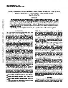
Figure 10. Sketch (not to scale) of the intersection between the wind-wind interacting region (represented by a cone) and the He+ region (represented by the orange circle) at phases around periastron. When the stars (white circles) are close enough, so that the wind-wind interacting region penetrates the He+ core in the primary wind, high-energy radiation produced in the shock cone (red line) can easily ionize He+ ions, and some of the radiation due to the eventual recombination processes will escape through the aperture of the ‘bore hole’. This will lead to an increasing in the production of He ii λ4686 photons.

60 10−>11 (2003.5) 11−>12 (2009.0) 12−>13 (2014.6)

(a)

0

Velocity (km s−1)

→

6950

Figure 9. (a) He ii λ4686 equivalent width curve for the last three events folded by 2022.9 d. (b) Doppler velocity measurements. The shaded region indicates the period where the peak velocity rapidly changes to more blue-shifted velocities, which repeated for the past three events. This kinematic behavior seems to be related only with P2.

2012; Madura et al. 2013). This is in agreement with the fact that the observed maximum Doppler velocity of the peak of the line profile is 400 . |V | . 450 km s−1 (see Figure 9b), which is comparable to the primary wind terminal velocity of 420 km s−1 (Groh et al. 2012a). This

4.1. A model for the variations in the He ii λ4686 equivalent width curve: opacity and geometry effects. Assuming that the He ii λ4686 emission is produced close to the apex of the shock cone, variations in the observed emission can, in principle, be explained by the increase in the total opacity along the line of sight to the emitting region, as the secondary moves deeper inside the dense primary wind. Intuitively, this mechanism would cause a gradual decrease (or increase, after periastron passage) of the observed flux that would depend on the extent and physical properties of the optically thick region in the extended primary wind, and also on the orbital orientation to the observer. This same approach was used by Okazaki et al. (2008) to show that the overall behavior of the RXTE X-ray light curve can be reproduced by assuming that the Xray emission comes from a point source located at the apex of the shock cone and prone to attenuation by the primary wind. Recently, Hamaguchi et al. (2014) sug-

The extraordinary He ii λ4686 in η Car EW0 (Å)

−30 −20

(a) Intrinsic He II λ4686 strength

width, EWsyn , at each orbital phase, was obtained using

from D−2 from bore hole effect Total

EWsyn (ϕ) = EW0 (ϕ) e−τA (ϕ) ,

−10

EWsyn(He II λ4686) (Å)

0 −3 −2 −1 0

(b) ω=0°

−3 −2 −1 0

(c) ω=90°

−3 −2 −1 0

(d) ω=180°

−3 −2 −1 0

(e) ω=270°

0.96

i=135° i=144° i=153°

0.98

1.00 ϕ (orbital)

1.02

13

1.04

Figure 11. (a) Intrinsic and (b–e) synthetic He ii λ4686 equivalent width curves. The basic assumption is that the He ii λ4686 emission comes from a region located at the apex and varies accordingly to the total column density in the line of sight to it as derived from 3D SPH simulations (D is the distance between the stars). The same intrinsic line strength was assumed for all orbit orientations. For each value of the longitude of periastron (ω), the different lines show the expected behavior of the equivalent width for the orbit inclinations (i) indicated in the legend. Variations in the equivalent width curve are more sensitive to ω than i. Based on these plots and the observations, we can promptly exclude 0◦ . ω . 180◦ and favor ω close to 270◦ .

gested that the variations across the spectroscopic events are composed of a combination of (1) occultation of the X-ray emitting region by the extended primary wind and (2) decline of the X-ray emissivity at the apex. In any case, opacity effects (either attenuation or occultation) can play an important role on the observed intensity of the radiation. Since the X-ray light curve shares some similarities with the He ii λ4686 equivalent width curve (both rise to a maximum before falling to a minimum when there is no emission at all), we tested the hypothesis that the variations in the He ii λ4686 equivalent width could also be the result of intrinsic emission attenuated by the extended primary wind. We used 3D SPH simulations of η Car from Madura et al. (2013) to calculate the total optical depth in the line of sight to the apex at each phase by using Z R τA (ϕ) = κe ρ dz, (1) z0 (ϕ)

where ρ and κe are, respectively, the mass density and the mass absorption coefficient of the material in the line of sight to the apex. The integration starts at the position of the apex at each phase z0 (ϕ) and goes up to the boundaries of the 3D SPH simulations, which, in this case, is a sphere with radius R = 154.5 AU. For the present work, we assumed that electron scattering is the dominant process for the attenuation of the radiation in the line of sight, which corresponds to κe = 0.34 cm2 g−1 . Therefore, under these circumstances, the synthetic equivalent

(2)

where EW0 (ϕ) is the intrinsic equivalent width (corresponding to the unattenuated flux). In the present work, we included only two mechanisms responsible for EW0 : (i) a continuous production of He ii λ4686 photons that varies reciprocally with the square of the distance D between the stars (i.e. in radiative conditions; see Fahed et al. 2011) and (ii) an additional, temporary contribution from the ‘bore hole’ effect that depends on how deep the apex of the shock cone penetrates inside the primary wind (see Madura & Owocki 2010). We included the contribution from the ‘bore hole’ effect because, near periastron, due to the highly eccentric orbit, the wind-wind interacting region penetrates into the inner regions of the primary wind, eventually exposing its He+ core19 . The contribution from this mechanism to the observed He ii λ4686 flux is proportional to how large the ‘bore hole’ is (see Figure 10). This assumption relies on the fact that high-energy radiation produced in the shock cone inside the He+ region (the red line between the cone and the sphere in Figure 10) can create He++ ions, whose recombination will produce He ii λ4686 photons. Some will eventually escape through the ‘bore hole’ and be detected by the observer. The radius rbh of the ‘bore hole’ is wavelengthdependent and varies with orbital phase. Considering the He+ region, rbh as a function of the orbital phase is given by 2 2 1/2 rbh (ϕ) = (RHe , (3) + − r (ϕ)) where r(ϕ) is the distance between the primary star and the plane formed by the aperture of the ‘bore hole’ (see Figure 10), given by 2 2 2 1/2 c2 z0 (ϕ) + (c2 (RHe + − z0 (ϕ)) + RHe+ ) , (4) c2 + 1 and c = tan α, where α is the half-opening angle of the cone formed by the wind-wind interacting region. In equations (3) and (4), RHe+ is the radius of the He+ region in the primary wind and z0 (ϕ) is the distance between the primary and the apex at a given orbital phase. Figure 11a shows the contribution from each mechanism to the total intrinsic equivalent width EW0 . The relative contribution was chosen so that the transition between the two regimes occurred smoothly, as required by the observations. Thus, by combining the intrinsic strength for the line emission with the total opacity in the line of sight, we were able to calculate a synthetic equivalent width curve for different orbit orientations. The results for selected orbital orientations are shown in Figure 11b–e.

r(ϕ) =

4.2. Modeling the He ii λ4686 equivalent width 4.2.1. The direct view of the central source Based on the comparison between the overall profile of the observed He ii λ4686 equivalent width curve from the past 3 cycles and those synthetic curves shown in 19 The He+ core has a radius of about 3 AU (Hillier et al. 2001; Groh et al. 2012a). Assuming an eccentricity of 0.9, the apex should be inside the He+ core for 0.98 . ϕ(orbital) . 1.02.

14

Teodoro et al.

1.4

i=144°; ω=243°

10−>11 (2003.5) 11−>12 (2009.0) 12−>13 (2014.6) −3

1.0

EW(He II λ4686) (Å)

Root mean square error (Å)

1.2

0.8

0.6

0.4

i=135°; ω=234° i=135°; ω=243° i=135°; ω=252° i=144°; ω=234° i=144°; ω=243° i=144°; ω=252° i=153°; ω=234° i=153°; ω=243° i=153°; ω=252°

−2

−1

0

0.2 −30

0 JD(obs)−JD(syn) (days)

30

Figure 12. Examples of the result of the comparison between the observed He ii λ4686 equivalent width curve and a series of synthetic curves from 3D SPH simulations with different orbital orientations (3 inclinations and 3 longitude of periastron). For each comparison, we shifted the models in time to determine the time of periastron passage. Each curve shows the least root mean square error as a function of the difference between the time of the observations, JD(obs), and that of the synthetic equivalent width curve, JD(syn), for the indicated orbit orientation. The best match occurred for i = 144◦ , ω = 243◦ (black solid line), and a time shift of about −4.0 d.

Figure 11, one can readily discard models with 0◦ . ω . 180◦ . Orientations with ω = 0◦ produce results that have excessively high optical depths before periastron passage and way too little after it. This orientation cannot reproduce the observed rise of the equivalent width before periastron passage and also overestimates its strength after it. Orientations with ω = 90◦ produce symmetrical profiles, which do not correspond to the observations. Orientations with ω = 180◦ can reproduce fairly well the observations before periastron but fail to reproduce the observed equivalent width after periastron (they underestimate P3). Regardless of the overall profile of the synthetic equivalent width curves, the crucial problem of models with 0◦ . ω . 180◦ is that they cannot reproduce the observed phase of the deep minimum – the week-long phase where the observed equivalent width is zero. Orientations with 230◦ . ω . 270◦ , on the other hand, seem to provide a good overall profile, as they predict an increase just before periastron passage followed by a rapid decrease to zero right after periastron passage, and the return to a lower (in modulo) equivalent width peak before fading away (P3). Thus, we focused our analysis on ω in this range. The duration of the interval when the synthetic equivalent width remains near zero (and whether it is ever reached) is also regulated by the orbital inclination. Thus, we compared the observations with 16 synthetic equivalent width curves obtained from the permutation of 4 values of orbital inclination (i ∈ {126◦, 135◦ , 144◦ , 153◦}) and 5 values of longitude of periastron (ω ∈ {225◦ , 234◦, 243◦ , 252◦ , 261◦}). Then we calculated the root mean square error (RMSE) between each model and the observations. The values for i and ω were obtained from a pre-defined grid within the 3D

0.96

0.98

1.00 ϕ (orbital)

1.02

1.04

Figure 13. Folded He ii λ4686 equivalent width curve compared with the best synthetic model (solid green line). The minimum RMSE occurs when the synthetic model is shifted by −4.0 d relative to the observations. Note that now the phase corresponds to the orbital phase.

SPH models. Also, note that the orbital plane is parallel to the plane of the sky for i = 0◦ or i = 180◦ , whereas for i = 90◦ or i = 270◦ they are perpendicular to each other. Thus, the set of orbital inclinations that we investigated in this work was chosen based on the premise that the orbital axis is aligned with the Homunculus polar axis (see Madura et al. 2012). For each model, we also searched for the time shift to be applied to the models that would result in the least root mean square value between the model and the observations. Examples of the results of this analysis are shown in Figure 12. The minimum RMSE was reached for an orbit orientation with {i = 144◦, ω = 243◦ } and a time shift JD(obs) − JD(syn) = −3.5 d. A comparison between the best model (with the derived time shift applied) and the observations is shown in Figure 13. Regarding the mean value and uncertainty of these results, statistical analysis showed that there are no significant differences between a model with a combination of i = 144◦ and 234◦ . ω . 252◦ . In fact, within the range of orbit orientations that we focused our analysis on, only these models resulted in RMSE significantly lower than the others at the 2σ level. Therefore, the mean values we adopted for i and ω are, respectively, 144◦ and 243◦ (coincidently equal to the best match), whereas the uncertainty on both values is defined by the step in the number of lines of sight used to produce the synthetic equivalent width curves from the 3D SPH models, which was set to 9◦ . In order to estimate the mean and uncertainty on the time shift, we adopted a sample composed of the time shift that resulted in the least RMSE for each one of the 16 models. The result was a mean time shift of −4.0 ± 2.0 d (the standard error is ±0.5 d). This means that periastron passage occurs 4 d after the onset of the He ii λ4686 deep minimum. 4.2.2. The event as viewed from high stellar latitudes An independent way to verify the reliability of our results would be analyzing the He ii λ4686 equivalent width curve from different viewing angles and comparing them

The extraordinary He ii λ4686 in η Car

20 As remarked by Stahl et al. (2005), the initial definition of FOS4, done using HST Faint Object Spectrograph images obtained in 1996-97, was a 0.5 arcsec wide region located 4.03 arcsec from the central source at PA = 135◦ . Given that the Homunculus nebula expands at an average rate of 0.03 arcsec yr−1 (e.g. Smith & Gehrz 1998), the current distance between FOS4 and the central source is about 4.5 arcsec

0 θ=90°

180 θ=180° 150

θ=0°

60

90

∆t

θ (°)

90

θ

θ=270° FOS4 position

120 ∆t (d)

with the results from the direct view of the central source. Fortunately, in the case of η Car, this is possible due to the bipolar reflection nebula – the Homunculus nebula – that surrounds the binary system. Each position along the Homunculus nebula ‘sees’ the central source along a different viewing angle (Smith et al. 2003b). An interesting position is the FOS4 (e.g. Davidson et al. 1995; Humphreys & HST-FOS eta Car Team 1999; Zethson et al. 1999; Rivinius et al. 2001; Stahl et al. 2005), a region about 1 arcsec2 in area located approximately 4.5 arcsec from the central source along the major axis of the Homunculus20 that is believed to reflect the spectrum originating at stellar latitudes close to the polar region (for comparison, the spectrum from the direct view of the central source seems to arise from intermediate stellar latitudes; see e.g. Smith et al. 2003b). We compared our results with those obtained at FOS4 by Mehner et al. (2015) using the same analysis that we did for the direct view of the central source. Note, however, that the time shift obtained from the observations at FOS4 needs to be corrected by the light travel time and the expansion of the reflecting nebula. We achieved this by using the Homunculus model derived by Smith (2006), to determine the necessary parameters of FOS4 (see Figure 14). In a coordinate system where a stellar latitude of θ = 90◦ corresponds to the pole of the receding NW lobe and θ = 270◦ corresponds to the pole of the approaching SE lobe, the spectrum reflected at FOS4 corresponds to a stellar latitude of θ(FOS4) = 258◦ , whereas the central source is viewed at θ0 = 229◦ . Figure 15 shows the search for the best match between the models and the observations. Since the orbital axis is closely aligned with the Homunculus polar axis, we investigated models corresponding to stellar latitudes θ ∈ {252◦ , 261◦, 270◦ } and ω ∈ {225◦, 243◦ , 252◦}. The best match was found for {θ = 261◦ , ω = 243◦} and a time shift of −21.0 d. This model resulted in a RMSE significantly lower (at the 2σ level) than any other one. Note that this time shift of 21 d, obtained empirically (Smith 2006), is consistent with previous estimates by Stahl et al. (2005) and Mehner et al. (2011) based on geometrical arguments. Since the observations at FOS4 were not as frequent as for the direct view, our analysis is subject to aliasing, which explains the high frequency oscillations observed in Figure 15. Despite that, we determined a mean time shift at FOS4 of −21.6 ± 1.3 d (the standard error is 0.4 d). Note that the smaller uncertainty of this result, when compared with the direct view of the central source, is not real. This is just an effect introduced by the fact that we used a smaller sample for the trial models for the polar region than for the direct view. Also, the variations between the trial models for the polar region are not as large as the ones for the direct view, which reduces the dispersion of the minimum RMSE (all the models for the pole region have similar time shift). The time shift we derived for FOS4 has to be corrected

15

180

270

30

0

−10

−5 0 5 Position along major axis (arcsec from the central source)

360 10

Figure 14. Time delay (∆t) and stellar latitude (θ) as a function of the projected position along the major axis of the Homunculus nebula. The inset illustration shows the the definition of the stellar latitude regarding the orientation of the Homunculus nebula. Values between 0◦ and 180◦ correspond to the NW lobe (θ = 90◦ being the NW pole), whereas latitudes between 180◦ and 360◦ correspond to the SE lobe (θ = 270◦ is the SE pole). In this system, the direct view of the central source corresponds to θ ≡ θ0 = 229◦ . The vertical dotted line indicates the FOS4 position, whereas the horizontal dashed lines indicate the corresponding values for ∆t = 17 d (left vertical axis) and θ = 258◦ (right vertical axis).

by light travel delay. Considering that the lobes are expanding at 650 km s−1 , the spectrum reflected at the FOS4 position would be delayed by ∆t = 17 d relative to the direct view of the central source. This means that 17 d, out of the observed −21.6 d, are due to light travel effect that must be taken into account in order to compare with the observations of the central source (again, the minus sign means periastron occurs after the onset of the He ii λ4686 deep minimum). Therefore, the best model for the observations at FOS4 results in an effective time shift of 17 d−21.6 d= −4.6 ± 0.4 d, which is in agreement with the results obtained from the direct view of the central source. Figure 16 shows the best model compared with the observations at FOS4 (corrected for light travel time). An interesting result is that when the ‘bore hole’ effect is included, the models overestimate the equivalent width at FOS4, which suggests that the contributions due to this mechanism is small at high stellar latitudes. This makes sense, given the fact that the contribution from the ‘bore hole’ effect will be significant toward where the cavity is pointing to (i.e. low and intermediate latitudes). The net result is that the ephemeris equation derived from the reflected observations at FOS4 (high stellar latitude), after correction by the travel time delay, is the same as for the direct view (intermediate stellar latitude). Therefore, the variations across the event for the He ii λ4686 seem to be ultimately determined by the high opacity in the line of sight to the He ii λ4686 emitting region during periastron passage, and not by a decrease in the intrinsic emission. 4.3. Ephemeris equation for periastron passage The results presented in this paper allowed us to determine the time of the periastron passage, T0 (2014.6),

16

Teodoro et al. (standard error), which is the result of error propagation from all the parameters used to determine the mean values shown in that equation. Table 6 summarizes all the orbital elements derived in this work and Figure 17 illustrates the orientation of the orbit projected onto the sky using the mean value for the orbital elements.

Root mean square error (Å)

0.4

0.3

θ=270°; ω=225° θ=270°; ω=243° θ=270°; ω=252° θ=261°; ω=225° θ=261°; ω=243° θ=261°; ω=252° θ=252°; ω=225° θ=252°; ω=243° θ=252°; ω=252°

0.2

−30

0 JD(obs)−JD(syn) (days)

30

Figure 15. Same as Figure 12, but for the position FOS4. At this position, we are looking at a spectrum originated at a stellar latitude θ that is being reflected off the Homunculus nebula. In this system, θ = 90◦ corresponds to the NW lobe pole, whereas θ = 270◦ corresponds to the SE lobe pole. The best match (black solid line) occurred for θ = 261◦ , ω = 243◦ , and a time shift of −21.0 d.

EW(He II λ4686) (Å)

−3

FOS4 10−>11 (2003.5) 11−>12 (2009.0) 12−>13 (2014.6) θ(FOS4)=261°; ω=243°

−2

−1 −2 0 0.99

1.00

1.01

−1

0

0.85

0.90

0.95 1.00 ϕ (orbital)

1.05

1.10

Figure 16. FOS4 observations from Mehner et al. (2015) corrected by the time delay (17 d). The green solid line corresponds to the best match model: θ(FOS4) = 261◦ and ω = 243◦ . The vertical dashed line indicates periastron passage.

from two different line of sights. For the direct view, T0 (2014.6) = 2456874.1 (standard deviation: ±2.8 d), whereas for the FOS4 T0 (2014.6) = 2456874.7 (standard deviation: ±2.3 d). Therefore, the time of periastron passage is given by JD(periastron passage) = 2456874.4 + 2022.7 E,

(5)

where E = (Φ − 13), Φ is the mean anomaly plus cycle21 , and 2022.7 corresponds to the mean period of the spectroscopic cycle. The time of periastron passage determined by equation (5) has an uncertainty of ±2.0 d 21 Following Groh & Damineli (2004), the cycle counting starts on JD = 2430578.4, corresponding to 1942 Aug 06, around the time when the first observed ‘low-excitation state’ due to a spectroscopic event was reported by Gaviola (1953).

4.4. The He ii λ4686/X-ray connection The comparison between the He ii λ4686 emission and the X-rays is inevitable because both are tracers of highenergy processes that might be interconnected. For example, X-rays produced in the wind-wind shock might be used to doubly-ionize neutral helium, in which case the He ii λ4686 emission should vary in a similar way to the X-rays. In η Car, the onset of the deep minimum, as determined from the observed He ii λ4686 and 2–10 keV X-ray emission light curves, occurs almost at the same time (see e.g. Teodoro et al. 2012; Hamaguchi et al. 2014). Incidentally, no significant changes in the time of the start of the deep minimum were observed over the past 3 cycles (Corcoran et al. 2016, in preparation). However, the recovery of the He ii λ4686 emission and the 2–10 keV X-ray flux occurs in a completely different way. So far, the observations support a scenario where the He ii λ4686 emission presents a recovery phase (after the deep minimum) that is stable and repeatable, whereas for the X-rays, recovery cannot be predicted. Indeed, in 1998.0 and 2003.5, the full recovery of the 2–10 keV X-ray flux occurred about 90 d after the onset of the deep minimum, but in 2009.0 it happened 30 d earlier than that. Even more intriguing, in 2014.6, the observations indicate that the recovery was intermediate between the 1998.0/2003.5 and 2009.0. Thus, the question is why does the He ii λ4686 and the X-ray emission enter the deep minimum at the same time but recover from it so differently? Are they connected? Hamaguchi et al. (2014) showed that the 2–10 keV Xray flux can be split into two regimes that behave differently in time: the soft (2–4 keV) and the hard X-ray band (4–8 keV). Those authors showed that the hard Xray flux (4–8 keV) drops to a minimum before the soft Xray flux (2–4 keV). In fact, by the time the latter reaches the minimum, the former is already recovering from it. Interestingly, He ii λ4686 emission enters the minimum phase about 4 d after the hard X-rays and about 12 d before the soft X-rays. This fact not only corroborates the idea that the He ii λ4686 emitting region is located in the vicinity of the apex (likely close to the hard X-ray emitting region), but is also consistent with the scenario proposed in this paper, in which the onset of the deep minimum is regulated by the orbital orientation and opacity effects, as the secondary moves toward periastron. In this scenario, emission from the apex should disappear first, followed by emission produced in regions gradually farther away from the WWC apex (i.e., downstream of the WWC structure). Therefore, the time when the deep minimum starts should be approximately the same for all features arising from spatially adjacent regions, as might be the case for He ii λ4686 and the X-rays (especially the hard band flux). Using the ephemeris from Hamaguchi et al. (2014), the deep minimum phase in the hard X-rays occurred, approximately, from JD = 2454843 through JD = 2454859, which suggests that superior conjunction would have

The extraordinary He ii λ4686 in η Car Table 6 Orbital elements derived in the present work, assuming orbital eccentricity ǫ = 0.9. Parameter Symbol Value or range Inclination i 135◦ –153◦ Longitude of periastron ω 234◦ –252◦ Period P 2022.7 ± 0.3a Time of periastron passage T0 (2014.6) 2456874.4 ± 1.3a a The error is the standard error of the mean.

10

N E

8

i = 144° Ω = 47° ω = 243°

ter, but not the former. For example, if the shock cone structure would switch from adiabatic to radiative during periastron passage, the result would be a substantial decrease of the hardest X-ray emission because the windwind interacting region would be cooler. The subsequent recovery of the X-ray emission would then depend on stochastic processes in order to re-establish the emission from the hot plasma in the wind-wind interaction region. This is not, however, the case for the He ii λ4686 emission because, during periastron passage, the He+ region of the primary star is exposed by the wind-wind interacting region, and, therefore, He ii λ4686 emission can still be produced during this phase, even if there is very low X-ray emission from the WWC region. 5. FINAL REMARKS

∆δ (mas)

6

4

2

0

3 AU

4

17

2

0 −2 ∆α (mas)

−4

−6

Figure 17. Orientation of the orbit of the secondary star as projected onto the sky using the mean value of the orbital elements derived in the present work. The arrows indicate the direction of the orbital motion. Note that the orbit is with respect to the primary star. The orbit was color-coded using the actual (not projected) distance between the stars, so that the orbit path becomes red as the stars are close to each other around periastron passage, and purple when they are at apastron. We adopted a distance of 2350 pc (Smith 2006).

occurred within this interval. According to equation (5), the 2009.0 periastron passage occurred on JD = 2454851.7, which falls approximately in the middle of the phase of minimum hard X-ray flux. Moreover, note that, for ω = 243◦, superior conjunction occurs very close to periastron passage, only 3.6 d later. Therefore, the orbital orientation as derived from Xray and He ii λ4686 emission are consistent. This is not surprising in the scenario we propose here. Indeed, close to periastron passages, we expect the hard X-ray and the He ii λ4686 to behave similarly (although they might not have a causal relation) because the apex of the shock cone is inside the primary He+ core where the He ii λ4686 emission is being produced at these phases. The soft X-rays, however, are produced in extended regions along the shock cone, and will eventually be blocked by the inner dense parts of the primary star at a later time. After periastron passage, the He ii λ4686 emission behaves differently from the X-rays likely due to intrinsic physical processes that inhibit or even shut off the lat-

Analysis of the data we have thus far indicate that only P2 has significantly increased in strength over the past two cycles (2009.0 and 2014.6). This is a robust result because we have daily measurements during the appearance of P2 for those epochs. However, except during the 2014.6 periastron passage, P1 and P3 have never been monitored with high cadence, which makes the comparison rather difficult because the equivalent width of the He ii λ4686 line shows variations at a wide range of timescales. One clear example is the absolute maximum strength of P3. The results from the 2009.0 analysis (including the additional data obtained with Hexapod/BESO) suggest that it is composed of a broad peak with a maximum absolute value of about 1.3 ˚ A, but the 2014.6 results indicate that P3 is actually a combination of broad and sharp components, with a maximum absolute value of 2 ˚ A. The broad component does repeat from cycle to cycle, but we cannot conclude the same for the narrow component, as we did not have enough time coverage during the time the narrow component seems to appear. Nonetheless, a caveat here is that short-timescale variations (less than a week) might occur due to local stochastic mechanisms, like the flares seen in X-rays before periastron passages. Such fluctuations cannot be easily distinguished from cyclic variations. Our model is especially sensitive to two parameters: (i) the total opacity in the line of sight to the apex and (ii) to the size of the He+ region in the primary wind. Hence, changes in these parameters will reflect on the overall behavior of the He ii λ4686 equivalent width curve. As a matter of fact, both parameters are ultimately connected to the mass-loss rate of the primary star. Changes in the primary’s mass-loss rate would result in variations in the timing and strength of the He ii λ4686 equivalent width curve (as already discussed in Madura et al. 2013). The repeatability of the overall behavior of the He ii λ4686 equivalent width over the past three cycles, as shown in this work, corroborates previous results that rule out large changes in mass-loss rate from the primary star over that time interval. 6. CONCLUSIONS We have monitored the He ii λ4686 emission line across the 2014.6 event using many ground-based telescopes as well as the HST. The main results derived from the analysis of the collected data are listed below.

18

Teodoro et al. • The period of 2022.9 ± 1.6 d, derived from He ii λ4686 monitoring, is in agreement with previous results; • Based on several different measurements across the electromagnetic spectrum, the mean orbital period is 2022.7 ± 0.3 d; • We have not detected statistically significant changes in the overall behavior of the He ii λ4686 equivalent width curve when comparing the events of 2009.0 and 2014.6 (best time sampled), which implies that the mechanism behind the production of EUV/soft X-rays photons must be relatively stable and recurrent; • When comparing each peak separately, between 2009.0 and 2014.6, P1 and the broad component of P3 have not changed significantly. Nevertheless, P2 has increased by 26%; • We have proposed a model to explain the variations of the He ii λ4686 equivalent width curve across each event. The model assumes two different mechanisms responsible for the intrinsic production of the line emission: (1) a component that is inversely proportional to the square of the distance between the two stars (always present throughout the orbit) and (2) another one associated with the ‘bore hole’ effect (present within about 30 d before and 30 d after periastron passage; negligible outside this time interval). The intrinsic emission was then convolved with the total optical depth in the line of sight to the He ii λ4686 emitting region (computed from 3D SPH simulations) to create a synthetic equivalent width that was compared with the observations; • Our model was able to successfully reproduce the overall behavior of the He ii λ4686 equivalent width curve from two very different viewing angles: a direct view and a polar view of the central source. The latter was possible due to observations from the FOS4 position on the SE lobe of the Homunculus nebula. This particular position is known for its capability of reflecting the spectrum of the central source produced at high stellar latitudes; • The best match between the models and observations from two different viewing angles (direct view of the central source and FOS4) suggests 234◦ . ω . 252◦ ; • We have determined the time of periastron passage by comparing the time shift required to give the best match between models (for which we know the orbital phase) and observations for two different lines of sight. The results suggest that both directions ‘see’ the periastron passage at the same time, about 4 d after the start of the deep minimum (as seen in the direct view of the central source);

In summary, our results suggest that the variations observed in the He ii λ4686 equivalent width curve across the spectroscopic events are governed by a combination of the orbit orientation regarding the observer and the

total optical depth in the line of sight to the emitting region. This is not a classical eclipse of the emitting region by the primary wind (the so-called ‘wind eclipse’ scenario). Instead, the ultimate nature of the spectroscopic event can be ascribed to the deep burial of the secondary star in the densest parts of the primary wind, so that emission from the vicinity of the apex of the shock cone cannot easily escape the system, resulting in a temporary decrease of the observed emission regardless of line of sight. As a reminder, the onset of the next He ii λ4686 deep minimum will occur on 2020 February 13. Periastron passage should occur four days later. ACKNOWLEDGMENTS During part ot this research, M. T. was supported by CNPq/MCT-Brazil through grant 201978/2012-1. A. D. thanks FAPESP for financial support through grant 2011/51680-6. F. W. thanks K. Davidson and R. Humphreys for their discussions leading to part of these observations. Some of the spectra were obtained under the aegis of Stony Brook University, whose participation has been supported by the office of the Provost. We are grateful to Pam Kilmartin and Fraser Gunn for helping with the observations at MJUO. A. F. J. M. is grateful to financial aid to NSERC (Canada) and FRQNT (Qu´ebec). N. D. R. gratefully acknowledges his CRAQ (Qu´ebec) postdoctoral fellowship. D. J. H. acknowledges support from HST-GO 12508.02-A. T. I. M. and C. M. P. R. are supported by an appointment to the NASA Postdoctoral Program at the Goddard Space Flight Center, administered by Oak Ridge Associated Universities through a contract with NASA. We are grateful to STScI for support with the observational schedule. This publication is based (in part) on spectroscopic data obtained through the collaborative Southern Astro Spectroscopy Email Ring (SASER) group.This research has made extensive use of NASA’s Astrophysics Data System, idl Astronomy User’s Library, and David Fanning’s idl Coyote library. This research has made use of the NASA Exoplanet Archive, which is operated by the California Institute of Technology, under contract with the National Aeronautics and Space Administration under the Exoplanet Exploration Program. We would like to thank an anonymous referee for constructive suggestions that improved the presentation of this work. Facilities: CTIO:1.5m (CHIRON), LNA:ZJ0.6m (Lhires iii), LNA:1.6m (Coud´e), SOAR (Goodman), MtJohn:1m (HERCULES), CASLEO (REOSC DC), OCA:Hexapod (BESO) REFERENCES Abraham Z., Falceta-Gon¸calves D., 2007, Monthly Notices of the Royal Astronomical Society, 378, 309 [1] Bauer D. F., 2012, Journal of the American Statistical Association, 67, 687 [3.3] Birnbaum Z. W., Tingey F. H., 1951, The Annals of Mathematical Statistics, 22, 592 [3.3] Clementel N., Madura T. I., Kruip C. J. H., Icke V., Gull T. R., 2014, Monthly Notices of the Royal Astronomical Society, 443, 2475 [1] Clementel N., Madura T. I., Kruip C. J. H., Paardekooper J. P., Gull T. R., 2015a, Monthly Notices of the Royal Astronomical Society, 447, 2445 [1] Clementel N., Madura T. I., Kruip C. J. H., Paardekooper J. P., 2015b, Monthly Notices of the Royal Astronomical Society, 450, 1388 [1]

The extraordinary He ii λ4686 in η Car Conover W. J., 1971, Practical nonparametric statistics. Vol. 15, New York, Wiley [3.3] Conti P. S., 1984, Observational Tests of the Stellar Evolution Theory. International Astronomical Union Symposium No. 105, 105, 233 [1] Corcoran M. F., Ishibashi K., Swank J. H., Petre R., 2001, The Astrophysical Journal, 547, 1034 [1] Corcoran M. F., Hamaguchi K., Pittard J. M., Russell C. M. P., Owocki S. P., Parkin E. R., Okazaki A., 2010, The Astrophysical Journal, 725, 1528 [1, 1] Damineli A., 1996, Astrophysical Journal Letters v.460, 460, L49 [1] Damineli A., Conti P. S., Lopes D. F., 1997, New Astronomy, 2, 107 [1] Damineli A., Stahl O., Kaufer A., Wolf B., Quast G., Lopes D. F., 1998, VizieR On-line Data Catalog, 413, 30299 [1, 2.2] Damineli A., Lopes D. F., Conti P. S., 1999, in Eta Carinae at The Millennium. p. 288 [1] Damineli A., et al., 2008a, Monthly Notices of the Royal Astronomical Society, 384, 1649 [1, 3.1, 4, 3.2] Damineli A., et al., 2008b, Monthly Notices of the Royal Astronomical Society, 386, 2330 [1] Davidson K., 1997, New Astronomy, 2, 387 [1] Davidson K., 2002, in The High Energy Universe at Sharp Focus: Chandra Science. p. 267 [1] Davidson K., Humphreys R. M., 1997, Annual Review of Astronomy and Astrophysics, 35, 1 [1] Davidson K., Ebbets D., Weigelt G., Humphreys R. M., Hajian A. R., Walborn N. R., Rosa M., 1995, Astronomical Journal (ISSN 0004-6256), 109, 1784 [4.2.2] Davidson K., Gull T., Walborn N. R., Gull T. R., 2002, in Eta Carinae: Reading the Legend. p. 7P [1] Davidson K., Mehner A., Humphreys R. M., Martin J. C., Ishibashi K., 2015, Astrophysical Journal, 801, L15 [1, 2, 7, 3.3.1] Durbin J. J. ., 1973 [3.3] Fahed R., et al., 2011, Monthly Notices of the Royal Astronomical Society, 418, 2 [4.1] Falceta-Gon¸calves D., Jatenco-Pereira V., Abraham Z., 2005, 357, 895 [1] Fisher R. A., 1925, Statistical methods for research workers. Edinburgh, London, Oliver and Boyd [3.3] Fisher R. A., 1935, The design of experiments. Edinburgh, London, Oliver and Boyde [3.3] Fuhrmann K., Chini R., Hoffmeister V. H., Lemke R., Murphy M., Seifert W., Stahl O., 2011, Monthly Notices of the Royal Astronomical Society, 411, 2311 [2.8] Gaviola E., 1950, Astrophysical Journal, 111, 408 [1] Gaviola E., 1953, Astrophysical Journal, 118, 234 [21] Groh J. H., Damineli A., 2004, Information Bulletin on Variable Stars, 5492, 1 [21] Groh J. H., et al., 2010, Astronomy and Astrophysics, 517, 9 [1] Groh J. H., Hillier D. J., Madura T. I., Weigelt G., 2012a, Monthly Notices of the Royal Astronomical Society, 423, 1623 [1, 4, 19] Groh J. H., Madura T. I., Hillier D. J., Kruip C. J. H., Kruip C. J. H., Weigelt G., 2012b, The Astrophysical Journal Letters, 759, L2 [1] Gull T. R., Madura T. I., Groh J. H., Corcoran M. F., 2011, The Astrophysical Journal Letters, 743, L3 [1] Hamaguchi K., et al., 2007, Astrophysical Journal, 663, 522 [1] Hamaguchi K., et al., 2014, The Astrophysical Journal, 784, 125 [4.1, 4.4, 4.4] Hearnshaw J. B., Barnes S. I., Kershaw G. M., Frost N., Graham G., Ritchie R., Nankivell G. R., 2002, Experimental Astronomy, 13, 59 [] Henley D. B., Corcoran M. F., Pittard J. M., Stevens I. R., Hamaguchi K., Gull T. R., 2008, The Astrophysical Journal, 680, 705 [1] Hillier D. J., Davidson K., Ishibashi K., Gull T., 2001, The Astrophysical Journal, 553, 837 [1, 19] Hillier D. J., et al., 2006, The Astrophysical Journal, 642, 1098 [1] Hollander M., Wolfe D. A. j. a., 1973, Nonparametric statistical methods. Vol. 17, New York, Wiley [3.3] Humphreys R. M., 1978, Astrophysical Journal, 219, 445 [1] Humphreys R. M., HST-FOS eta Car Team 1999, Eta Carinae At The Millennium, 179, 107 [4.2.2] Kashi A., Soker N., 2008, Monthly Notices of the Royal Astronomical Society, 390, 1751 [1] Kashi A., Soker N., 2009, Publications of the Astron. Soc. of Australia, 397, 1426 [1] Kashi A., Soker N., 2015, eprint arXiv:1508.03576 [1] Knuth D. E., 2011, Choice Reviews Online, 48, 48 [3.3] Madura T. I., Groh J. H., 2012, The Astrophysical Journal Letters, 746, L18 [1]

19

Madura T. I., Owocki S. P., 2010, The Interferometric View on Hot Stars (Eds. Th. Rivinius & M. Cur´ e) Revista Mexicana de Astronom´ıa y Astrof´ısica (Serie de Conferencias) Vol. 38, 38, 52 [1, 4.1] Madura T. I., Gull T. R., Owocki S. P., Groh J. H., Okazaki A. T., Russell C. M. P., 2012, Monthly Notices of the Royal Astronomical Society, 420, 2064 [1, 4.2.1] Madura T. I., et al., 2013, Monthly Notices of the Royal Astronomical Society, 436, 3820 [1, 1, 4, 4.1, 5] Marsaglia G., Tsang W. W., Wang J., 2003, Journal of Statistical Software, 8, 1 [3.3] Martin J. C., Davidson K., Humphreys R. M., Hillier D. J., Ishibashi K., 2006, The Astrophysical Journal, 640, 474 [1, 1, 2, 4] Mehner A., Davidson K., Ferland G. J., Humphreys R. M., 2010, The Astrophysical Journal, 710, 729 [1] Mehner A., Davidson K., Martin J. C., Humphreys R. M., Ishibashi K., Ferland G. J., 2011, The Astrophysical Journal, 740, 80 [1, 1, 3.1, 4, 4.2.2] Mehner A., et al., 2015, Astronomy and Astrophysics, 578, A122 [1, 1, 4.2.2, 16] Moffat A. F. J., Corcoran M. F., 2009, The Astrophysical Journal, 707, 693 [1] Nielsen K. E., Corcoran M. F., Gull T. R., Hillier D. J., Hamaguchi K., Ivarsson S., Lindler D. J., 2007, The Astrophysical Journal, 660, 669 [1] Okazaki A. T., Owocki S. P., Russell C. M. P., Corcoran M. F., 2008, Monthly Notices of the Royal Astronomical Society: Letters, 388, L39 [1, 4.1] Parkin E. R., Pittard J. M., Corcoran M. F., Hamaguchi K., Stevens I. R., 2009, Monthly Notices of the Royal Astronomical Society, 394, 1758 [1] Parkin E. R., Pittard J. M., Corcoran M. F., Hamaguchi K., 2011, The Astrophysical Journal, 726, 105 [1] Pittard J. M., Corcoran M. F., 2002, Astronomy and Astrophysics, 383, 636 [1] Plavchan P., Jura M., Kirkpatrick J. D., Cutri R. M., Gallagher S. C., 2008, The Astrophysical Journal Supplement Series, 175, 191 [3.1] R Core Team 2014, R: A Language and Environment for Statistical Computing. R Foundation for Statistical Computing, Vienna, Austria [3.3] Richardson N. D., Gies D. R., Henry T. J., Fern´ andez-Laj´ us E., Okazaki A. T., 2010, The Astronomical Journal, 139, 1534 [1, 2.1] Richardson N. D., Gies D. R., Gull T. R., Moffat A. F. J., St-Jean L., 2015, The Astronomical Journal, 150, 109 [1, 2.1] Rivinius T., Wolf B., Stahl O., Kaufer A., 2001, in Eta Carinae and Other Mysterious Stars: The Hidden Opportunities of Emission Spectroscopy. p. 29 [4.2.2] Russell C. M. P., 2013, PhD thesis, ProQuest Dissertations And Theses; Thesis (Ph.D.)–University of Delaware, University of Delaware [1] Scholz F. W., Stephens M. A., 1987, Journal of the American Statistical Association, 82, 918 [3.3] Smith N., 2006, The Astrophysical Journal, 644, 1151 [4.2.2, 17] Smith N., Gehrz R. D., 1998, The Astronomical Journal, 116, 823 [20] Smith N., Gehrz R. D., Hinz P. M., Hoffmann W. F., Hora J. L., Mamajek E. E., Meyer M. R., 2003a, The Astronomical Journal, 125, 1458 [1] Smith N., Davidson K., Gull T. R., Ishibashi K., Hillier D. J., 2003b, The Astrophysical Journal, 586, 432 [1, 4.2.2] Stahl O., Weis K., Bomans D. J., Davidson K., Gull T. R., Humphreys R. M., 2005, Astronomy and Astrophysics, 435, 303 [4.2.2, 20] Steffen W., et al., 2014, Monthly Notices of the Royal Astronomical Society, 442, 3316 [1] Steiner J. E., Damineli A., 2004, The Astrophysical Journal, 612, L133 [1, 1] Stellingwerf R. F., 1978, Astrophysical Journal, 224, 953 [3.1] Teodoro M., Damineli A., Sharp R. G., Groh J. H., Barbosa C. L., 2008, Monthly Notices of the Royal Astronomical Society, 387, 564 [1] Teodoro M., et al., 2012, The Astrophysical Journal, 746, 73 [1, 1, 2, 4, 4.4] Teodoro M., Madura T. I., Gull T. R., Corcoran M. F., Hamaguchi K., 2013, The Astrophysical Journal Letters, 773, L16 [1, 2.4] Tokovinin A., Fischer D. A., Bonati M., Giguere M. J., Moore P., Schwab C., Spronck J. F. P., Szymkowiak A., 2013, Publications of the Astronomical Society of the Pacific, 125, 1336 [2.1] Verner E., Bruhweiler F., Gull T., 2005, The Astrophysical Journal, 624, 973 [1]

20

Teodoro et al.

Zanella R., Wolf B., Stahl O., 1984, Astronomy and Astrophysics (ISSN 0004-6361), 137, 79 [1]

Zethson T., Zethson T., Johansson S., Davidson K., Humphreys R. M., Ishibashi K., Ebbets D., 1999, Astronomy and Astrophysics, 344, 211 [4.2.2]

APPENDIX Table 7 lists all the 2014.6 measurements presented in this paper, as well as information about the quality and wavelength coverage of each spectrum used. Table 7 He ii λ4686 emission line measurements and spectral characteristics of the data obtained during the international campaign to monitor the 2014.6 periastron passage. Velocity of Wavelength the peak ∆va coverage EW −1 −1 b ˚ JD-2450000 Observatory (A) (km s ) (km s ) SNR (˚ A) 4967.47314 +0.16 ± 0.08 −10 185.7 1579 3499–6168 SOAR 4978.45698 +0.16 ± 0.08 −28 185.8 1079 3497–6167 SOAR 5012.50000 +0.03 ± 0.03 −678 39.5 955 4560–4826 HST 5171.50000 +0.20 ± 0.03 −678 39.5 629 4560–4826 HST 5495.50000 +0.35 ± 0.03 −678 39.5 334 4560–4826 HST 5689.50746 −0.23 ± 0.08 −23 92.5 350 3509–4839 SOAR 5729.53926 +0.06 ± 0.08 +522 92.1 342 3516–4841 SOAR 5768.49673 +0.12 ± 0.08 +514 92.0 353 3517–4840 SOAR 5856.82809 +0.08 ± 0.08 +526 92.0 307 3517–4839 SOAR 5885.50000 +0.16 ± 0.03 −678 39.5 272 4560–4826 HST 5893.79688 −0.24 ± 0.08 −668 92.1 396 3509–4832 SOAR 5930.77193 −0.06 ± 0.08 −59 92.0 379 3513–4836 SOAR 5955.81938 +0.14 ± 0.08 −672 92.0 250 3518–4841 SOAR 5982.61373 +0.11 ± 0.08 +526 91.9 346 3517–4839 SOAR 5989.68923 +0.01 ± 0.13 +530 3.5 640 4505–4755 CTIO 5993.75221 +0.04 ± 0.13 +530 3.5 620 4505–4755 CTIO 6001.72621 +0.08 ± 0.13 +530 3.5 678 4505–4755 CTIO 6003.63393 +0.05 ± 0.08 +514 92.0 287 3518–4840 SOAR 6013.68632 +0.22 ± 0.13 −684 3.5 594 4505–4755 CTIO 6039.52767 +0.02 ± 0.08 +525 92.2 422 3511–4836 SOAR 6079.49884 +0.03 ± 0.08 +515 92.1 299 3519–4843 SOAR 6116.49641 −0.13 ± 0.08 +530 92.0 279 3521–4844 SOAR 6136.46326 +0.08 ± 0.08 +527 92.2 289 3515–4841 SOAR 6218.50000 +0.22 ± 0.03 −358 39.5 368 4560–4826 HST 6221.89057 +0.20 ± 0.13 +530 3.5 584 4505–4755 CTIO 6236.84632 −0.06 ± 0.13 −684 3.5 548 4505–4755 CTIO 6238.87015 −0.04 ± 0.13 −684 3.5 410 4505–4755 CTIO 6246.79354 +0.01 ± 0.08 +521 92.0 323 3517–4839 SOAR 6248.81477 −0.10 ± 0.13 +530 3.5 606 4505–4755 CTIO 6254.88181 −0.19 ± 0.13 −684 3.5 558 4505–4755 CTIO 6260.78284 −0.05 ± 0.13 +530 3.5 433 4505–4755 CTIO 6275.81899 +0.28 ± 0.13 −684 3.5 673 4505–4755 CTIO 6278.81225 +0.26 ± 0.08 +518 92.0 333 3516–4839 SOAR 6289.79792 +0.16 ± 0.13 −684 3.5 788 4505–4755 CTIO 6346.69729 +0.09 ± 0.08 −673 91.9 439 3520–4841 SOAR 6361.58149 −0.24 ± 0.08 +526 91.9 327 3518–4839 SOAR 6361.64473 +0.12 ± 0.13 +530 3.1 742 4505–4755 CTIO 6401.58757 −0.07 ± 0.13 +530 3.1 772 4505–4755 CTIO 6417.58964 −0.09 ± 0.13 +530 3.1 675 4505–4755 CTIO 6428.48444 −0.03 ± 0.08 +522 92.3 460 3511–4837 SOAR 6428.64093 −0.03 ± 0.13 +131 3.8 2046 4575–4800 CTIO 6452.52706 −0.05 ± 0.08 +31 92.2 357 3514–4840 SOAR 6488.47634 −0.19 ± 0.08 +14 91.9 484 3516–4838 SOAR 6538.50000 +0.10 ± 0.03 −17 39.5 265 4560–4826 HST 6607.84573 +0.12 ± 0.13 +530 3.1 497 4505–4755 CTIO 6612.86785 −0.22 ± 0.13 +324 3.1 577 4505–4755 CTIO 6613.83605 −0.34 ± 0.08 +15 91.1 420 3632–4941 SOAR 6655.76290 +0.01 ± 0.15 −1 47.2 615 6398–6720 SOAR 6656.70393 −0.09 ± 0.08 −30 3.1 1225 4283–4961 CTIO 6659.70988 −0.08 ± 0.13 −29 3.1 690 4505–4755 CTIO 6664.67479 −0.17 ± 0.13 +530 3.1 607 4505–4755 CTIO 6670.78253 −0.01 ± 0.13 −31 3.1 657 4505–4755 CTIO 6672.83764 −0.04 ± 0.13 −71 3.1 766 4505–4755 CTIO 6677.75915 −0.17 ± 0.13 +12 3.1 625 4505–4755 CTIO 6687.70761 −0.10 ± 0.13 −37 3.1 755 4505–4755 CTIO 6690.69063 −0.18 ± 0.13 −6 3.1 800 4505–4755 CTIO 6697.72572 −0.27 ± 0.08 −2 3.1 743 4505–4755 CTIO 6698.77338 −0.17 ± 0.08 +55 3.7 1814 4505–4755 CTIO 6701.62899 −0.03 ± 0.13 +10 99.7 399 4575–4800 OPD (Lhires iii) 6701.74483 −0.26 ± 0.03 +136 46.1 184 4571–5052 OPD (Coud´ e) 6705.50000 −0.18 ± 0.03 +22 39.5 374 4396–4894 HST 6710.66775 −0.10 ± 0.03 +14 3.1 911 4560–4826 CTIO 6712.69246 −0.23 ± 0.13 −7 3.1 614 4505–4755 CTIO 6718.70977 −0.15 ± 0.13 −45 3.1 680 4505–4755 CTIO 6724.59005 −0.22 ± 0.13 −11 3.7 1944 4505–4755 CTIO 6725.56888 −0.12 ± 0.13 −103 3.1 700 4575–4800 CTIO 6729.55975 −0.23 ± 0.13 −126 3.0 946 4505–4755 CTIO 6730.60581 −0.23 ± 0.15 +527 26.6 655 6399–6720 CASLEO 6732.60351 −0.20 ± 0.13 −111 3.0 899 4505–4755 CTIO 6739.49790 −0.22 ± 0.13 −42 91.3 934 4540–4760 SOAR 6739.54616 −0.22 ± 0.13 −42 3.1 828 4505–4755 CTIO 6746.51736 −0.39 ± 0.35 −37 3.1 628 3627–4940 CTIO 6750.53884 −0.30 ± 0.13 +2 3.1 642 4505–4755 CTIO 6754.55102 −0.31 ± 0.13 −44 3.1 702 4505–4755 CTIO 6759.52573 −0.25 ± 0.13 −17 91.4 486 4505–4755 SOAR 6763.55612 −0.33 ± 0.13 −36 29.1 1082 4505–4755 CASLEO 6765.58734 −0.40 ± 0.35 +7 3.0 878 3625–4940 CTIO 6766.54334 −0.25 ± 0.13 −61 3.1 987 4540–4760 CTIO 6767.50868 −0.35 ± 0.13 +14 3.1 908 4505–4755 CTIO 6769.52337 −0.23 ± 0.13 −1 46.1 517 4505–4755 OPD (Coud´ e) 6772.43126 −0.54 ± 0.13 −73 100.1 201 4505–4755 OPD (Lhires iii)

The extraordinary He ii λ4686 in η Car

JD-2450000 6774.54408 6775.46760 6777.53611 6781.47143 6784.84146 6786.50087 6786.80812 6787.50338 6787.80222 6789.57938 6791.55016 6793.39493 6793.43162 6793.51309 6795.44909 6795.44909 6795.50702 6796.46794 6796.66742 6797.51150 6797.56402 6800.41794 6800.46206 6801.49770 6802.50447 6803.52719 6805.46847 6805.48993 6806.52963 6807.61259 6809.45843 6810.48189 6811.48702 6812.45066 6813.40174 6813.42771 6814.41074 6814.43755 6816.43650 6816.43650 6817.50000 6818.42255 6818.50425 6820.41744 6821.80127 6822.38703 6822.45982 6823.45482 6823.53806 6823.86265 6824.51692 6825.44362 6825.46968 6825.50553 6826.42638 6826.45073 6826.85107 6827.40873 6827.43762 6827.77608 6828.40903 6829.50184 6830.39501 6830.39501 6831.47240 6832.50051 6833.37832 6833.37832 6833.50054 6835.36656 6835.53378 6836.36515 6836.49685 6837.38253 6838.51346 6839.46217 6839.50001 6840.45062 6840.46309 6840.49851 6841.39145 6842.43257 6843.38235 6844.41845 6845.46145 6847.45640 6847.47008 6850.38667 6850.50978 6850.96486

EW (˚ A) −0.33 ± 0.13 −0.53 ± 0.13 −0.45 ± 0.13 −0.31 ± 0.13 −0.49 ± 0.13 −0.56 ± 0.13 −0.78 ± 0.08 −0.62 ± 0.13 −0.80 ± 0.08 −0.80 ± 0.13 −0.63 ± 0.08 −0.57 ± 0.13 −0.52 ± 0.13 −0.61 ± 0.13 −0.63 ± 0.13 −0.63 ± 0.13 −0.72 ± 0.13 −0.52 ± 0.13 −0.72 ± 0.13 −0.80 ± 0.35 −0.69 ± 0.13 −0.87 ± 0.13 −0.65 ± 0.13 −0.64 ± 0.13 −0.79 ± 0.13 −0.70 ± 0.13 −0.93 ± 0.13 −1.01 ± 0.13 −0.84 ± 0.13 −0.85 ± 0.13 −0.79 ± 0.13 −0.69 ± 0.13 −0.79 ± 0.13 −0.60 ± 0.13 −0.76 ± 0.13 −0.89 ± 0.13 −0.66 ± 0.13 −0.62 ± 0.13 −0.73 ± 0.13 −0.77 ± 0.13 −0.94 ± 0.13 −0.91 ± 0.13 −0.67 ± 0.03 −0.89 ± 0.13 −1.09 ± 0.13 −1.14 ± 0.13 −1.32 ± 0.22 −1.20 ± 0.13 −1.12 ± 0.35 −1.16 ± 0.13 −1.47 ± 0.13 −1.27 ± 0.22 −1.26 ± 0.13 −1.59 ± 0.13 −1.30 ± 0.13 −1.30 ± 0.13 −1.37 ± 0.13 −1.42 ± 0.13 −1.21 ± 0.22 −1.51 ± 0.13 −1.38 ± 0.13 −1.57 ± 0.22 −1.31 ± 0.13 −1.32 ± 0.13 −1.72 ± 0.13 −1.43 ± 0.13 −1.15 ± 0.35 −1.20 ± 0.13 −1.34 ± 0.13 −1.35 ± 0.13 −1.17 ± 0.13 −1.52 ± 0.13 −1.33 ± 0.13 −1.40 ± 0.13 −1.65 ± 0.13 −1.86 ± 0.13 −1.98 ± 0.13 −2.25 ± 0.13 −2.53 ± 0.13 −2.43 ± 0.13 −2.08 ± 0.35 −2.52 ± 0.13 −2.26 ± 0.13 −2.07 ± 0.13 −1.82 ± 0.13 −1.62 ± 0.13 −1.98 ± 0.13 −1.87 ± 0.13 −1.82 ± 0.35 −1.93 ± 0.13

Table 7 — Continued Velocity of the peak ∆va (km s−1 ) (km s−1 ) SNR b −152 3.1 784 +28 3.7 1968 +71 3.7 1819 −105 3.1 911 −33 3.2 1252 −43 3.7 2346 −43 3.2 1041 −46 3.7 1774 −54 3.2 1390 −135 26.5 519 −135 3.1 1017 −159 100.2 585 −153 100.2 260 −163 26.5 1712 −185 100.3 114 −185 100.3 114 −174 3.1 971 −175 93.7 1262 −158 100.3 103 −159 100.3 564 −174 26.5 462 −93 46.9 433 −102 3.1 838 −94 3.1 737 +3 3.7 1702 −100 3.1 1034 −27 100.3 388 −4 100.3 275 −46 3.7 460 +68 3.7 490 −4 3.7 2494 −94 3.1 868 −260 3.7 2121 −166 99.3 151 −239 99.9 567 −230 99.9 193 −176 99.9 732 −165 99.9 186 −205 99.8 393 −207 99.8 280 −178 39.5 359 −174 99.8 233 −185 3.1 888 −148 102.4 546 −67 3.2 901 −136 102.4 525 −106 91.2 2197 −58 99.9 522 −68 3.1 772 −62 3.2 960 −58 3.1 1085 −89 99.9 719 −90 99.9 379 −68 3.7 2021 −104 99.9 924 −83 99.9 339 −74 3.2 886 −113 99.9 835 −107 99.9 622 −119 3.2 1263 −67 102.4 602 −42 3.1 481 −11 99.9 637 −23 99.9 660 −8 91.3 411 −32 3.1 908 −63 99.9 800 −60 99.9 238 −38 3.7 1941 −159 102.4 615 −132 3.1 489 −159 102.4 997 −149 3.1 758 −184 100.0 1368 −196 3.7 1813 −172 100.0 395 −169 3.7 2037 −149 100.0 360 −124 91.3 1422 −121 3.7 2212 −73 100.2 350 −136 102.4 1203 −183 102.4 704 −171 100.3 616 −267 3.1 737 −155 3.7 1097 −167 91.2 2228 −206 102.4 658 −182 3.1 789 −185 72.2 747

Wavelength coverage (˚ A) 4461–4959 4571–5055 4505–4755 4575–4800 4575–4800 4505–4755 4586–4818 4575–4800 4586–4817 4575–4800 4586–4817 4540–4760 4505–4755 4569–5053 4569–5053 4540–4760 4570–5055 4570–5055 4505–4755 3593–4940 4565–5049 4556–5040 4540–4760 4035–5176 4505–4755 4505–4755 4575–4800 4505–4755 4568–5052 4568–5052 4575–4800 4575–4800 4575–4800 4505–4755 4575–4800 4574–5054 4573–5056 4573–5056 4573–5055 4573–5055 4573–5055 4573–5055 4560–4826 4587–5069 4505–4755 4577–5055 4586–4818 4577–5055 3626–4938 4575–5057 4505–4755 4589–4818 4505–4755 4574–5057 4574–5057 4575–4800 4574–5057 4575–5057 4586–4818 4574–5057 4574–5057 4586–4818 4577–5055 4505–4755 4575–5057 4575–5057 3626–4938 4505–4755 4574–5057 4574–5057 4575–4800 4577–5055 4505–4755 4577–5055 4505–4755 4576–5058 4575–4800 4576–5059 4575–4800 4575–5059 3627–4939 4575–4800 4574–5058 4577–5055 4577–5055 4577–5061 4505–4755 4575–4800 3628–4939 4577–5055

21

Observatory CTIO CTIO CTIO CTIO MJUO CTIO MJUO CTIO MJUO CASLEO CTIO OPD (Lhires iii) OPD (Lhires iii) CASLEO OPD (Lhires iii) OPD (Lhires iii) CTIO SOAR OPD (Lhires iii) OPD (Lhires iii) CASLEO OPD (Coud´ e) CTIO CTIO CTIO CTIO OPD (Lhires iii) OPD (Lhires iii) CTIO CTIO CTIO CTIO CTIO OPD (Lhires iii) OPD (Lhires iii) OPD (Lhires iii) OPD (Lhires iii) OPD (Lhires iii) OPD (Lhires iii) OPD (Lhires iii) HST OPD (Lhires iii) CTIO OPD (Lhires iii) MJUO OPD (Lhires iii) SOAR OPD (Lhires iii) CTIO MJUO CTIO OPD (Lhires iii) OPD (Lhires iii) CTIO OPD (Lhires iii) OPD (Lhires iii) MJUO OPD (Lhires iii) OPD (Lhires iii) MJUO OPD (Lhires iii) CTIO OPD (Lhires iii) OPD (Lhires iii) SOAR CTIO OPD (Lhires iii) OPD (Lhires iii) CTIO OPD (Lhires iii) CTIO OPD (Lhires iii) CTIO OPD (Lhires iii) CTIO OPD (Lhires iii) CTIO OPD (Lhires iii) SOAR CTIO OPD (Lhires iii) OPD (Lhires iii) OPD (Lhires iii) OPD (Lhires iii) CTIO CTIO SOAR OPD (Lhires iii) CTIO SASER

22

Teodoro et al.

JD-2450000 6851.38473 6852.40542 6852.49418 6853.37790 6853.49939 6854.80431 6854.89023 6855.35972 6855.45860 6855.47657 6855.77993 6855.86527 6855.94552 6856.36061 6856.45431 6856.46706 6856.47223 6856.87230 6857.45360 6858.40539 6858.45238 6858.48475 6859.46549 6859.49223 6860.38078 6860.86021 6861.39604 6862.40458 6862.86946 6863.46562 6863.47455 6864.46694 6864.46759 6864.93373 6865.87094 6866.51214 6867.41180 6867.46441 6867.46611 6867.85881 6868.39812 6868.84061 6869.38458 6869.46329 6869.82462 6869.85601 6869.94795 6870.38838 6870.45625 6870.46307 6871.42775 6871.46362 6871.49786 6871.50000 6871.91627 6872.37893 6872.46439 6872.85370 6872.93725 6873.38419 6873.46368 6873.48259 6874.38414 6874.45527 6874.47893 6874.85828 6874.93947 6875.38311 6875.47747 6876.38636 6876.45922 6876.48405 6877.40420 6877.48745 6877.94054 6878.39833 6878.48279 6878.93662 6878.98294 6879.39884 6879.46777 6880.46780 6880.48893 6880.93207 6881.46594 6882.46242 6883.46622 6883.47352 6883.83814 6883.92037 6884.93750 6885.42504 6885.46393 6885.87352 6886.47066

EW (˚ A) −2.30 ± 0.13 −2.77 ± 0.15 −2.93 ± 0.13 −3.29 ± 0.15 −2.79 ± 0.13 −2.57 ± 0.30 −3.31 ± 0.13 −2.95 ± 0.15 −3.09 ± 0.30 −2.79 ± 0.15 −2.69 ± 0.15 −3.10 ± 0.47 −2.74 ± 0.15 −3.17 ± 0.13 −3.16 ± 0.15 −3.51 ± 0.13 −2.35 ± 0.30 −3.25 ± 0.47 −3.23 ± 0.15 −3.27 ± 0.15 −3.07 ± 0.13 −2.76 ± 0.13 −2.70 ± 0.35 −3.03 ± 0.30 −2.73 ± 0.15 −2.82 ± 0.15 −2.47 ± 0.15 −2.65 ± 0.13 −2.64 ± 0.15 −2.41 ± 0.13 −2.51 ± 0.13 −2.37 ± 0.30 −2.16 ± 0.15 −2.22 ± 0.15 −1.69 ± 0.15 −0.93 ± 0.13 −0.88 ± 0.30 −0.55 ± 0.15 −0.69 ± 0.13 −0.30 ± 0.15 −0.44 ± 0.13 +0.19 ± 0.15 −0.39 ± 0.13 −0.28 ± 0.15 −0.48 ± 0.15 +0.35 ± 0.13 +0.07 ± 0.35 −0.24 ± 0.35 +0.18 ± 0.13 +0.21 ± 0.15 −0.03 ± 0.15 +0.18 ± 0.15 −0.11 ± 0.13 +0.09 ± 0.13 +0.22 ± 0.13 −0.03 ± 0.35 +0.07 ± 0.15 +0.64 ± 0.13 +0.31 ± 0.15 +0.02 ± 0.15 +0.06 ± 0.13 +0.15 ± 0.35 +0.12 ± 0.15 −0.04 ± 0.15 +0.14 ± 0.15 +0.17 ± 0.15 −0.25 ± 0.13 +0.14 ± 0.13 +0.13 ± 0.35 −0.00 ± 0.15 −0.02 ± 0.13 +0.03 ± 0.13 −0.18 ± 0.03 +0.12 ± 0.03 −0.02 ± 0.15 −0.25 ± 0.15 −0.39 ± 0.15 +0.04 ± 0.13 −0.12 ± 0.13 −0.60 ± 0.15 −0.45 ± 0.15 −0.41 ± 0.15 −0.49 ± 0.13 +0.08 ± 0.13 −0.44 ± 0.03 −0.49 ± 0.15 −0.51 ± 0.13 −0.38 ± 0.13 +0.29 ± 0.03 −0.47 ± 0.15 −0.10 ± 0.15 −0.42 ± 0.15 −0.46 ± 0.13 −0.32 ± 0.03 −0.44 ± 0.13

Table 7 — Continued Velocity of the peak ∆va (km s−1 ) (km s−1 ) SNR b −194 102.4 875 −217 102.4 599 −200 25.9 1543 −171 102.4 949 −163 25.7 329 −164 3.2 732 −176 46.4 409 −229 102.4 339 −198 3.1 1288 −220 25.8 667 −207 3.2 1071 −229 56.5 785 −215 206.1 1265 −263 102.4 449 −263 3.7 2879 −234 91.4 1033 −275 25.8 356 −243 52.4 409 −266 3.1 1229 −275 102.4 622 −271 3.1 1329 −300 25.8 521 −272 3.1 999 −295 25.7 777 −252 102.4 802 −251 45.8 619 −309 102.4 585 −304 102.4 575 −296 46.3 65 −326 3.1 1162 −304 91.3 1498 −323 91.3 1031 −335 3.1 1180 −326 44.4 1271 −313 44.1 430 −371 3.0 1215 −398 100.3 501 −396 3.0 770 −390 91.3 670 −368 3.2 733 −374 100.2 379 −681 63.4 67 −336 100.3 663 −98 91.2 331 +530 3.2 779 +350 63.1 85 −668 208.6 267 −677 100.2 590 +530 3.1 796 +516 91.5 1174 +523 100.3 489 +530 3.1 729 −397 26.0 391 −678 39.5 503 +528 47.9 919 +531 102.4 581 −684 3.1 1381 +3 60.8 79 +514 207.5 379 +531 102.4 592 −684 3.1 1000 +523 25.9 667 +531 102.4 300 +530 3.1 1193 +374 27.0 845 +529 72.1 118 −76 207.7 3778 +531 102.4 415 +528 26.0 687 −90 102.4 446 −231 3.1 387 +114 26.0 836 −56 102.4 615 −674 26.0 603 −212 119.2 542 −90 102.4 572 −94 3.1 758 −104 116.8 416 −27 146.3 93 −67 102.4 213 −28 3.1 969 −60 3.1 951 −263 102.4 86 −32 106.3 202 −48 3.1 1034 −55 3.1 1248 −28 3.1 439 −423 27.0 887 −26 3.2 600 −131 44.5 364 −158 122.0 423 −79 102.4 84 −100 3.1 806 −72 145.8 303 −38 3.1 967

Wavelength coverage (˚ A) 4505–4755 4574–4792 4577–5055 4614–5359 4577–5055 4540–4760 4577–5055 6396–6720 4540–4760 4781–6681 6397–6720 4586–4818 4570–4791 4577–5055 6397–6720 4505–4755 4540–4760 4586–4818 4570–4791 4159–4913 4577–5055 4575–4800 3625–4938 4540–4760 4570–4791 6020–6768 6019–6768 4505–4755 5736–6824 4577–5055 4505–4755 4540–4760 4773–6676 6397–6720 6397–6720 4505–4755 4540–4760 6397–6720 4577–5055 4578–4791 4577–5055 6397–6720 4577–5055 6398–6720 4578–4792 4505–4755 3625–4938 3626–4938 4505–4755 4570–4792 4570–4788 6355–6724 4505–4755 4574–5058 4505–4755 3627–4939 4586–4818 4575–5059 6397–6720 4524–5100 4574–5058 3628–4938 4586–4818 4526–5098 4174–4925 6061–6804 4574–5058 4505–4755 3624–4939 6061–6803 4574–5059 4505–4755 4540–4760 4560–4826 4572–4792 6060–6805 6060–6806 4577–5055 4505–4755 4561–5101 4175–4925 6060–6808 4577–5055 4505–4755 4540–4760 5745–7657 4577–5055 4505–4755 4540–4760 4488–5059 4167–4923 6065–6804 4577–5055 4540–4760 4577–5055

Observatory OPD (Lhires iii) OPD (Lhires iii) CASLEO OPD (Lhires iii) CASLEO MJUO SASER OPD (Lhires iii) CTIO CASLEO MJUO SASER SASER OPD (Lhires iii) CTIO SOAR CASLEO SASER CTIO OPD (Lhires iii) CTIO CASLEO CTIO CASLEO OPD (Lhires iii) SASER OPD (Lhires iii) OPD (Lhires iii) SASER CTIO SOAR SOAR CTIO SASER SASER CTIO OPD (Lhires iii) CTIO SOAR MJUO OPD (Lhires iii) SASER OPD (Lhires iii) SOAR MJUO SASER SASER OPD (Lhires iii) CTIO SOAR OPD (Lhires iii) CTIO CASLEO HST SASER OPD (Lhires iii) CTIO SASER SASER OPD (Lhires iii) CTIO CASLEO OPD (Lhires iii) CTIO CASLEO SASER SASER OPD (Lhires iii) CASLEO OPD (Lhires iii) CTIO CASLEO OPD (Lhires iii) CASLEO SASER OPD (Lhires iii) CTIO SASER SASER OPD (Lhires iii) CTIO CTIO OPD (Lhires iii) SASER CTIO CTIO CTIO CASLEO MJUO SASER SASER OPD (Lhires iii) CTIO SASER CTIO

The extraordinary He ii λ4686 in η Car

EW (˚ A) −0.47 ± 0.13 −0.60 ± 0.03 −0.43 ± 0.13 −0.47 ± 0.03 −0.51 ± 0.15 −0.60 ± 0.15 −0.70 ± 0.13 −0.68 ± 0.13 −0.72 ± 0.15 −0.52 ± 0.15 −0.75 ± 0.15 −0.89 ± 0.13 −1.24 ± 0.13 −0.60 ± 0.13 −0.54 ± 0.13 −1.18 ± 0.15 −1.07 ± 0.13 −1.11 ± 0.13 −1.08 ± 0.13 −1.22 ± 0.22 −1.36 ± 0.03 −1.56 ± 0.15 −1.64 ± 0.15 −1.71 ± 0.15 −2.14 ± 0.13 −1.64 ± 0.13 −2.02 ± 0.15 −2.03 ± 0.13 −2.03 ± 0.13 −1.68 ± 0.13 −1.59 ± 0.15 −1.42 ± 0.13 −1.15 ± 0.22 −1.51 ± 0.13 −1.58 ± 0.15 −1.46 ± 0.13 −1.45 ± 0.13 −1.35 ± 0.15 −1.02 ± 0.13 −1.26 ± 0.13 −1.08 ± 0.47 −1.05 ± 0.15 −1.04 ± 0.15 −0.76 ± 0.47 −0.86 ± 0.15 −0.77 ± 0.47 −1.07 ± 0.47 −0.71 ± 0.13 −0.83 ± 0.47 −0.72 ± 0.13 −0.99 ± 0.47 −0.90 ± 0.47 −1.17 ± 0.13 −0.71 ± 0.47 −0.78 ± 0.15 −0.67 ± 0.13 −0.31 ± 0.47 −0.67 ± 0.47 −0.65 ± 0.13 −0.40 ± 0.47 −0.24 ± 0.15 −0.02 ± 0.13 +0.04 ± 0.47 −0.09 ± 0.13 −0.27 ± 0.13 +0.01 ± 0.47 +0.03 ± 0.15 −0.03 ± 0.13 −0.04 ± 0.47 −0.06 ± 0.13 −0.03 ± 0.13 +0.03 ± 0.15 −0.01 ± 0.13 −0.07 ± 0.15 +0.05 ± 0.13 −0.00 ± 0.13 −0.00 ± 0.15 +0.02 ± 0.15 +0.03 ± 0.15

JD-2450000 6887.46157 6888.38076 6888.93513 6889.40109 6889.46464 6890.38792 6890.84660 6891.37832 6892.37992 6892.93822 6893.40410 6894.39500 6895.80517 6895.81175 6895.93682 6896.79905 6896.82025 6897.79931 6898.80025 6899.41741 6899.79987 6900.39932 6900.80626 6901.80112 6902.37996 6902.79568 6902.92365 6903.39135 6903.80951 6904.80022 6905.40209 6905.81433 6905.94347 6906.38324 6906.80165 6906.83424 6907.37853 6907.80059 6907.80869 6908.38139 6908.87070 6909.38647 6910.38143 6910.80338 6910.82866 6911.30601 6911.38002 6911.80060 6911.95672 6912.94395 6914.94813 6915.24671 6915.94736 6916.94919 6917.78979 6919.26677 6923.24250 6924.23432 6924.23432 6928.50000 6938.83294 6941.90973 6942.91028 6943.90679 6949.24499 6950.87840 6951.87621 6952.86748 6953.88255 6954.83416 6955.86423 6956.87673 6957.89313 6958.86680 6959.84998 6960.73148 6961.85099 6964.86782 6965.86504 a Resolution element. b Signal-to-noise ratio per resolution element.

Table 7 — Continued Velocity of the peak ∆va (km s−1 ) (km s−1 ) SNR b +11 3.7 755 −33 102.4 818 −14 115.4 168 −21 102.4 597 +527 26.0 338 −10 102.4 505 +468 59.0 140 +35 102.4 643 +35 102.4 1030 −32 106.2 207 +12 102.4 456 −21 102.4 380 −22 3.2 908 −198 71.8 218 +3 95.0 112 −54 3.2 1023 −99 71.1 296 −39 3.2 810 −30 3.2 955 −56 102.4 248 −20 3.2 931 −44 102.4 262 −23 3.2 1231 −9 3.2 956 −56 102.4 540 −3 3.2 750 +30 70.9 169 −33 102.4 410 −21 3.2 1365 −33 3.2 920 −79 102.4 253 −25 3.2 605 −14 100.8 351 −21 102.4 419 −23 3.2 864 −56 102.4 494 −79 102.4 317 −18 3.2 846 −52 68.9 282 −44 102.4 159 −11 3.2 457 −33 102.4 272 −67 102.4 279 −57 70.6 470 −67 102.4 1054 −60 398.8 79 −79 102.4 378 −90 102.4 652 −123 94.5 314 −180 89.7 226 −145 100.2 421 −126 473.3 124 −128 98.0 792 −57 117.3 114 −102 102.4 645 −85 453.1 477 −81 54.3 77 −192 137.9 84 −95 70.4 97 −37 39.5 462 −102 102.4 708 −643 3.0 157 −90 3.1 213 −74 3.1 595 −81 36.3 121 −179 3.1 1301 −114 3.1 1268 −81 3.1 725 +3 3.1 1128 −13 3.1 796 +223 3.1 982 −27 3.1 1281 +3 3.1 914 +84 3.1 850 −44 3.1 951 −44 102.4 599 +33 3.1 1009 −3 3.1 904 −5 3.1 1244

Wavelength coverage (˚ A) 4505–4755 4540–4760 4577–5055 4540–4760 4165–4917 6054–6798 4577–5055 4505–4755 4165–4917 4628–5808 6054–6798 4577–5055 4505–4755 4505–4755 4577–5055 4163–4919 4505–4755 4505–4755 4505–4755 4540–4760 4591–4817 4581–4792 4163–4919 6054–6798 4577–5055 4505–4755 4573–5755 4505–4755 4575–4800 4577–5055 4163–4919 4577–5055 4540–4760 4577–5055 4489–5031 4577–5055 4577–5055 4163–4919 4577–5055 4577–5055 4586–4818 4619–5199 4163–4919 4586–4817 4622–5195 4586–4818 4586–4818 4577–5055 4586–4818 4577–5055 4586–4818 4586–4818 4577–5055 4586–4818 4618–5190 4577–5055 4586–4817 4586–4817 4577–5055 4589–4818 4163–4919 4577–5055 4586–4818 4577–5055 4577–5055 4586–4818 4598–5169 4577–5055 4586–4818 4577–5055 4577–5055 4595–5168 4577–5055 4282–5799 4577–5055 4577–5055 4164–4918 4164–4918 4168–4915

23

Observatory CTIO OPD (Lhires iii) SASER OPD (Lhires iii) CASLEO OPD (Lhires iii) SASER OPD (Lhires iii) OPD (Lhires iii) SASER OPD (Lhires iii) OPD (Lhires iii) MJUO SASER SASER MJUO SASER MJUO MJUO OPD (Lhires iii) MJUO OPD (Lhires iii) MJUO MJUO OPD (Lhires iii) MJUO SASER OPD (Lhires iii) MJUO MJUO OPD (Lhires iii) MJUO SASER OPD (Lhires iii) MJUO OPD (Lhires iii) OPD (Lhires iii) MJUO SASER OPD (Lhires iii) MJUO OPD (Lhires iii) OPD (Lhires iii) SASER OPD (Lhires iii) SASER OPD (Lhires iii) OPD (Lhires iii) SASER SASER SASER SASER SASER SASER OPD (Lhires iii) SASER SASER SASER SASER HST OPD (Lhires iii) CTIO CTIO CTIO SASER CTIO CTIO CTIO CTIO CTIO CTIO CTIO CTIO CTIO CTIO OPD (Lhires iii) CTIO CTIO CTIO